5. Atmosphere configurations
There are a number of atmospheric models which can run within CESM. While CAM is the basic atmospheric model within CESM, there are several models with significant extensions to CAM which may also be run within CESM. The available atmospheric models in CESM3 are:
CAM: Community Atmosphere Model
CAM-chem: Community Atmosphere Model with Chemistry
WACCM: Whole Atmosphere Community Climate Model
WACCM-X: Whole Atmosphere Community Climate Model with thermosphere and ionosphere extension
CAM Simple Models: Atmospheres with idealized physics, idealized surfaces, single columns, and offline drivers.
Each of these models has a number of standalone CAM configurations provided to run them. These configurations are implemented in the CIME framework via compsets as discussed in CESM2 Component Sets. The predefined compsets have the support levels:
Scientific support: Specific compset/resolution pairs which have had significant, multi-year runs made and have been studied scientifically. It is important to note that resolutions which are not listed, are not scientifically supported, have not had tunings performed and should not be used for scientific studies without careful examination of the results.
Functional support: One or more tests for this compset have been made using at least one resolution. Extensive scientific study has not been performed. No attempts have been made to validate the scientific quality of these runs and tunings have NOT been performed on them.
Unsupported: These compsets are setup as a convenience for various reasons and they are not supported for science runs. If a user decides to use one of these compsets, they must also supply the
--run-unsupportedflag tocreate_newcase. These compsets may not even compile and run successfully as they are not regularly tested.
The compsets for standalone CAM are the F, P, and Q compsets (F, P, and Q are the first letters of the compset aliases). They are broadly defined as follows:
F compsets use CAM and active Land (CTSM) with prescribed Sea-Surface Temperatures (SSTs) and sea-ice extent (other components are stubs).
P compsets use only the CAM component configured to run only the radiation code driven by data collected from a previous run. This configuration is called PORT – Parallel Offline Radiation Tool.
Q compsets use CAM with a data ocean. CAM is configured to run aquaplanet simulations with either prescribed ocean (QP) or slab ocean(QS).
This chapter will discuss some of the atmospheric compsets in more detail, but a complete listing of all compsets is found at CESM2 Component Configurations (compsets). The complete listing of grid resolutions can be found at CESM2 Grid Resolutions.
5.1. Grids
5.1.1. Uniform grids
CAM7 does not support running with the Finite Volume dycore. It must be run using the Spectral Element (SE) dycore. The following describes some of the uniform resolution grids available:
ne3pg3_ne3pg3_mt232
Approximately 10 degree CAM-SE-CSLAM
ne30_ne30_mt232
Approximately 1 degree CAM-SE
ne30pg3_ne30pg3_mt232
Approximately 1 degree CAM-SE-CSLAM
ne30pg2_ne30pg2_mt232
Approximately 1 degree CAM-SE-CSLAM with a lower resolution physics grid (approximately 1.5 degrees)
ne120pg3_ne120pg3_mt13
Approximately 1/4 degree CAM-SE-CSLAM
ne120pg2_ne120pg2_mt12
Approximately 1/4 degree CAM-SE-CSLAM with a lower resolution physics grid (approximately 3/8 degree)
In physics grid (pg) configurations using CAM-SE-CSLAM each element is divided in 3x3 (pg3) or 2x2 (pg2) quasi-uniform resolution physics columns. The pg3 and pg2 configurations are documented in Herrington et al. (2019a) and Herrington et al. (2019b), respectively.
5.1.2. Variable resolution grids
The following variable resolution grids have been tested with the listed compsets:
ne0CONUSne30x8_ne0CONUSne30x8_mt12
Approximately 1/4 degree resolution over the Contiguous United States and approximately 1 degree elsewhere
compsets?
ne0ARCTICne30x4_ne0ARCTICne30x4_mt12
Approximately 1/4 degree resolution over Greenland and approximately 1 degree elsewhere
compsets?
ne0ARCTICGRISne30x8_ne0ARCTICGRISne30x8_mt12
Approximately 1/8 degree resolution over Greenland, otherwise identical to the ne0ARCTICne30x4 grid elsewhere
compsets?
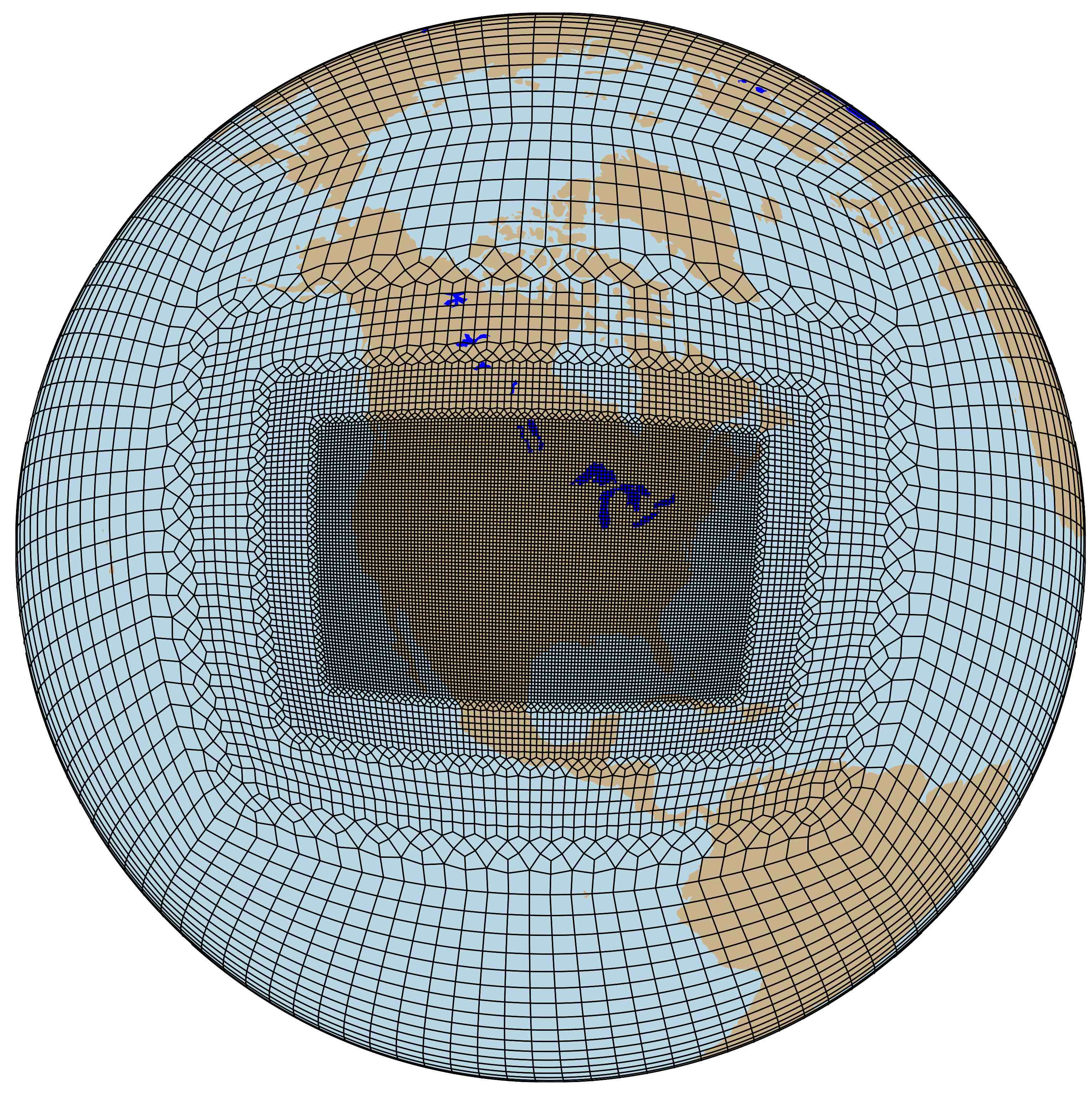
CONUS Grid
The CONUS variable resolution grid is a 1 degree horizontal resolution grid with a regional refinement of 1/8 degree resolution over the continential United States.
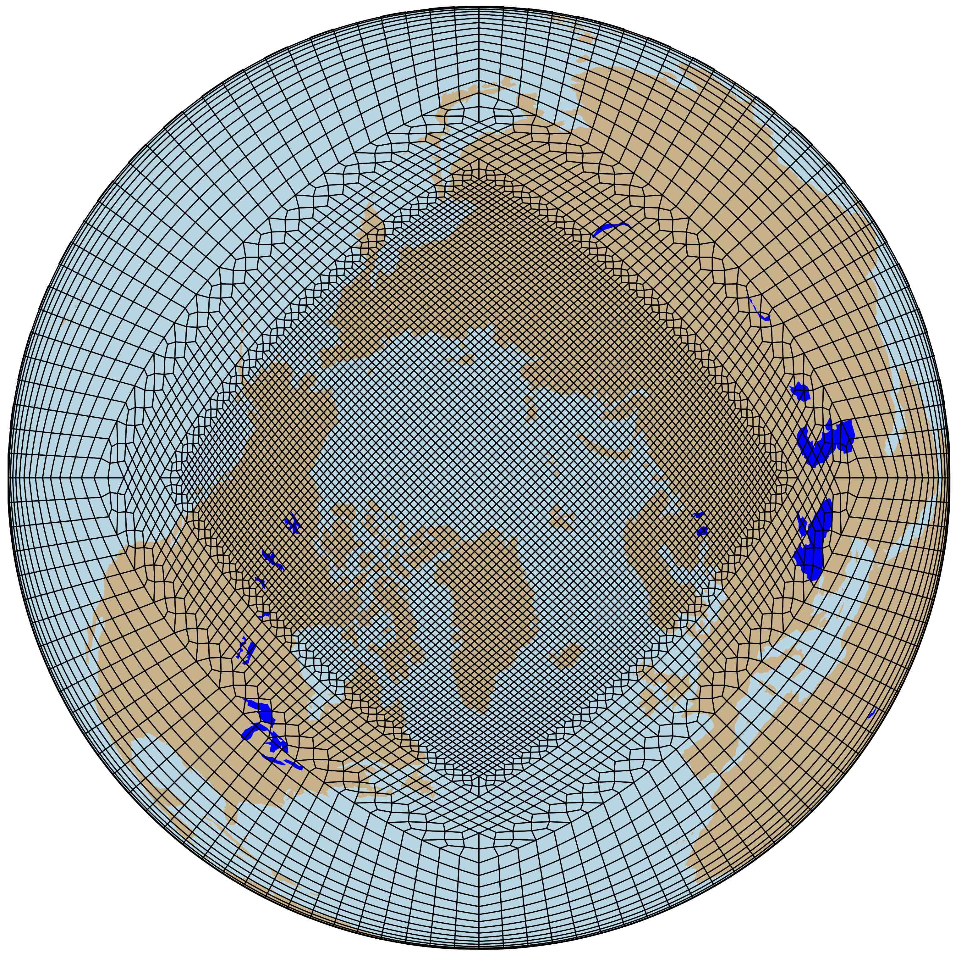
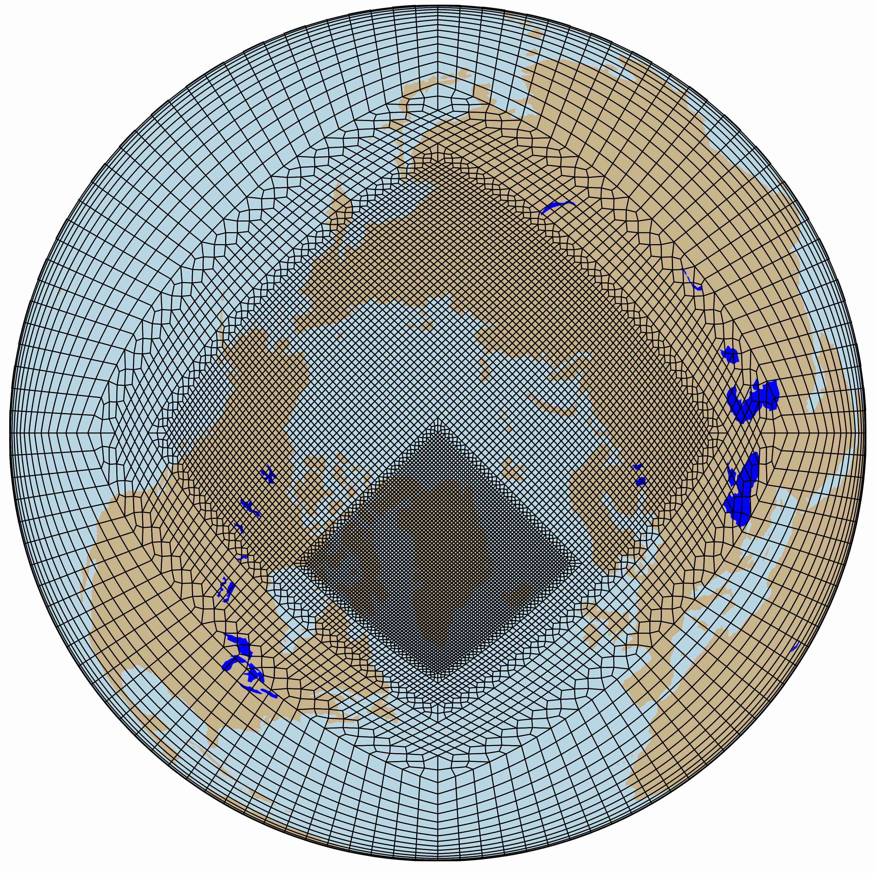
ARCTIC Grids
Two variable resolution grids are available for the Artic region. The ARCTIC grid, which is a 1 degree horizontal resolution grid with regional refinement of 1/4 degree resolution over the broader Arctic region and the ARCTICGRIS grid which additionally refines a patch covering the Greenland with 1/8 degree resolution.
|
|
5.2. CAM compsets
CAM7 has a number of compsets/resolutions which are supported scientifically. These compsets are detailed in the following table. A specific compset may be listed below, but unless the resolution is also listed, that compset/resolution combination is not scientifically supported. Different resolutions exhibit different behavior and as a result require different tunings. The scientifically supported designation is limited to the specific compset/resolution pairs listed in the following tables.
CAM7 is released with two supported model tops. The “low top” version (CAM7-LT) has the top at about 40-km which is the same as the previous CAM4, CAM5, CAM6 models, but has 58 vertical layers and thus a higher vertical resolution than the previous models which used 26, 30, and 32 layers respectively. The “medium top” version (CAM7-MT) has the top at about 80-km and uses 93 vertical layers.
Scientifically supported compsets
FHISTC_LTso
Historical CAM7-LT
ne30pg3_ne30pg3_mt232
1979 to 2015
FHISTC_MTso
Historical CAM7-MT
ne30pg3_ne30pg3_mt232
1979 to 2015
Tested compsets
F1850
CAM6, 1850 climatology
f10_f10_mt232
F2000climo
CAM6, 2000 climatology
f19_f19_mt232, mpasa480_mpasa480_mt232, mpasa120_mpasa120_mt232, C96_C96_mt232
F2010climo
CAM6, 2010 climatology
f09_f09_mt232,
FHIST
CAM6, Historical
f19_f19_mt232, f09_f09_mt232, f10_f10_mt232, ne3pg3_ne3pg3_mt232, ne0ARCTICne30x4_ne0ARCTICne30x4_mt12
FHIST_BDRD
CAM6 with carbon cycle, Historical
f09_f09_mt232
FHIST_C5
CAM5, Historical
f10_f10_mt232, f19_f19_mt232, ne3pg3_ne3pg3_mt232
F1850_C4
CAM4, 1850 climatology
ne3pg3_ne3pg3_mt232
FHIST_C4
CAM4, Historical
ne16pg3_ne16pg3_mt232
5.3. CAM-chem compsets
Tested compsets
In CESM3 new compsets have been included and existing ones have been slightly changed with regard to starting dates and available resolutions. In particular, new resolutions for running the spectral element dynamical core have been added as have new compsets that use meteorological nudging using MERRA2 on CESM model levels. Starting dates have been changed to start in 2010-2014 using default CMIP6 emissions, besides for the regional refined grid over CONUS. Other anthropogenic and biomass burning emissions are available covering different periods. New emission regridding tools are available. These compsets have functional support and have been tested with the listed grids and time periods:
FC2010climo
Climatological CAM6-chem using TS1 chemistry, 1 deg horizontal resolution, different dycores, averaged SSTs, emis, lower boundary conditions (2005-2015)
f09_f09_mg17, ne30_ne30_mg17, ne30pg3_ne30pg3_mg17
2010
FCHIST
Historical CAM6-chem using TS1 chemistry, 1 deg horizontal resolution, different dycores, CMIP6 emissions, coupled to interactive land and MEGAN2.1
f09_f09_mt232, ne30_ne30_mt232, ne30pg3_ne30pg3_mt232
2010-2014
FCnudged
As FCHIST, but nudged to U,V,T from MERRA2 analsysis with a 50-hours interpolated to CAM6 (32) model levels
f09_f09_mt232, ne30_ne30_mt232, ne30pg3_ne30pg3_mt232, ne0CONUSne30x8_ne0CONUSne30x8_mt12 (for 2013 only)
2010-2014
FCts2nudged
As FCnudged, but using TS2 chemistry
f09_f09_mt232, ne30_ne30_mt232, ne30pg3_ne30pg3_mt232, ne0CONUSne30x8_ne0CONUSne30x8_mt12 (for 2013 only)
2010-2014
FCSD
Historical CAM6-chem 1deg compset using MERRA2 analsysis with a 50-hour relaxation, using MERRA vertical levels
f09_f09_mg17
1980-2015
5.4. WACCM compsets
Scientifically supported compsets
Scientifically supported WACCM atmosphere configurations use TSMLT1 chemistry (see chemical mechanisms ) and the ne30pg3_ne30pg3_mt232 grid for the listed time periods:
FW1850
Pre-industrial control WACCM6 using 1-degree SE dycore, TSMLT1, CMIP6 piControl emissions, year 1850 SSTs, coupled to interactive land and MEGAN2.1
1850
FWHIST
Historical WACCM6 using 1-degree SE dycore, TSMLT1, CMIP6 emissions, historical SSTs, coupled to interactive land and MEGAN2.1
1974-2015
FW2000
Year 2000 WACCM6 1deg compset using 1-degree SE dycore, TSMLT1, year 2000 CMIP6 emissions, year 2000 SSTs, coupled to interactive land and MEGAN2.1
2000
FWSD
Historical SD-WACCM6 using GEOS5 analysis with a 50-hour relaxation, TSMLT1, CMIP6 emissions, historical SSTs, coupled to interactive land and MEGAN2.1
2005-2015
FWscHIST
Historical SC-WACCM6 using 1-degree SE dycore, specified chemistry, historical SSTs
1976-2015
Tested compsets
Tested WACCM atmosphere configurations use middle atmosphere (MA) and
middle atmosphere plus D-region (MAD) chemistry (see chemical
mechanisms ) and the ne30pg3_ne30pg3_mt232
grid for the listed time periods:
FWmaHIST
Historical WACCM6 using 1-degree SE dycore, MA chemistry, CMIP6 emissions, historical SSTs, coupled to interactive land and MEGAN2.1
1974-2015
FWmadHIST
Historical WACCM6 using 1-degree SE dycore, MAD chemistry, CMIP6 emissions, historical SSTs, coupled to interactive land and MEGAN2.1
1974-2015
FWmaSD
Historical SD-WACCM6 using GEOS5 analysis with a 50-hour relaxation, MA chemistry, CMIP6 emissions, historical SSTs, coupled to interactive land and MEGAN2.1
2005-2015
FWmadSD
Historical SD-WACCM6 using GEOS5 analysis with a 50-hour relaxation, MAD chemistry, CMIP6 emissions, historical SSTs, coupled to interactive land and MEGAN2.1
2005-2015
5.5. WACCM-X compsets
Scientifically supported compsets
Scientifically support WACCM-X compsets use the ne30pg3_ne30pg3_mt232 grid for the listed time periods:
FXHIST
Historical WACCM-X based on CAM4 using 1 degree SE dycore, MA chemistry, CCMI emissions, historical SSTs, coupled to land, prescribed ice, river
2000-2015
FX2000
Year 2000 WACCM-X based on CAM4 1 degree SE dycore, using MA chemistry, year 2000 CCMI emissions and SSTs, coupled to interactive land, prescribed ice, river
2000
FXSD
Historical SD-WACCM-X based on CAM4 using 1 degree SE dycore, MERRA1 with a 50-hour relaxation, MA chemistry, CCMI emissions, historical SSTs, coupled to interactive land, prescribed ice, river
2000-2015
5.6. CAM Simple Models
There are many simpler configurations in which CAM can be run. These include:
Idealized physics/chemistry
Aquaplanet
SCAM - Single column model
PORT - Parallel Offline Radiation Tool
Note
For more information on running these compsets and for sample outputs to aid in verifying that the model is running correctly see the CESM Simpler Models project.
5.6.1. Ideal physics compsets
FADIAB
Generic adiabatic configuration. All physics turned off.
FHS94
Dry Held-Suarez as described in Held and Suarez (1994).
FTJ16
Moist Held-Suarez following Thatcher and Jablonowski (2016). Based on the Held-Suarez physics configuration but including a simple representation of the large scale condensation of moisture and the diabatic heating.
FKESSLER
Ulrich et al. (2014) baroclinic wave with Kessler (1969) microphysics and the Lauritzen et al. (2015) terminator toy chemistry.
FGRAYRAD
Idealized gray radiation configuration following the protocol of Frierson et al (2006).
Note that the ideal physics compsets can be run with any of the dycores
provided in CAM (FV, FV3, SE, SE-CSLAM and MPAS). They are set up by
default to use the CAM7-LT vertical grid (40 km top with 58 layers). There
are many more compset/grid combinations than are tested by CAM’s regression
tests. An untested combination will cause create_newcase to stop with
the following message:
STOP:
This compset and grid combination is untested in CESM.
Override this warning with the --run-unsupported option to create_newcase.
To continue using the untested combination just reissue the
create_newcase command and append the “run-unsupported” flag:
% ./create_newcase --case ... --compset ... --res ... --run-unsupported
5.6.2. CAM aquaplanet
The aquaplanet configuration allows the user to run CAM above an entirely ocean covered surface. The standard protocol for aquaplanet experiments comes from the AquaPlanet Experiment project (APE; Neale & Hoskins [2], Williamson et al. [3]). The advantage of an aquaplanet configuration is that it allows the user to run the full CAM parameterization suite while retaining much simpler surface conditions than the complex combination of land, ocean, and sea-ice in the real world. The CAM5 aquaplanet configuration is described in detail by Medeiros et al. [1].
Prescribed SST
The aquaplanet compsets use the data ocean model to provide the prescribed
SST. By default the SST pattern is the APE “QOBS” option (provided by the
component _DOCN%AQP3_), which is used in APE and CFMIP protocols.
There are compsets for running with all the available CAM physics packages:
QPC7 – Prescribed SST Aquaplanet using CAM7-LT
QPC6 – Prescribed SST Aquaplanet using CAM6
QPC5 – Prescribed SST Aquaplanet using CAM5
QPC4 – Prescribed SST Aquaplanet using CAM4
Several compset/grid combinations are tested by CAM’s regression test
suite. But if a combination of interest is not tested, then supplying the
--run-unsupported option to create_newcase will allow the desired
case to be created. The tested combinations have spun up initial
conditions files available. If a combination of interest doesn’t have an
appropriate initial file, then build-namelist will fail with the message:
CAM build-namelist - ERROR: No default value found for ncdata
In this case the easiest way forward is to start the run from analytic initial conditions as described in the section “Use analytic initial conditions”.
Alternate Prescribed SST
All of the APE SST profiles are available from the data ocean model. To use them invoke the long compset name with the user compset option, e.g.:
% ./create_newcase --case ... --compset 2000_CAM50_SLND_SICE_DOCN%AQP7_SROF_SGLC_SWAV \
  --res ... --run-unsupported
Note
You may see a message “Did not find an alias or longname compset match…”. This message may be ignored.
This example uses the 3KEQ SST pattern, which is specified with
_DOCN%AQP7_ in the compset name. The analytical SST profiles are
defined in the source code
$COMP_ROOT_DIR_OCN/docn_datamode_aquaplanet_mod.F90. Also note this
example switched to CAM5 physics by specifying “CAM50” in the compset
name. The --run-unsupported option is required.
User-specified Prescribed SST dataset
An arbitrary SST dataset can be specified instead of the default APE SST. To do that, start by setting up the case with the desired compset/grid combination, and then change the data ocean mode and specify the file. For example, from the case directory modify the following CIME variables:
% ./xmlchange DOCN_MODE=sst_aquapfile
% ./xmlchange DOCN_AQP_FILENAME=/my_data/sst.nc
Where /my_data/sst.nc is the user-supplied SST file, which follows the
same conventions as SST files used for F compsets.
Aquaplanet with Slab-Ocean Model
The data ocean model has a slab-ocean configuration which may be used with the aquaplanet configuration. The following SOM-Aquaplanet compsets are available:
QSC6 – Slab-Ocean Aquaplanet for CAM6
QSC5 – Slab-Ocean Aquaplanet for CAM5
QSC4 – Slab-Ocean Aquaplanet for CAM4
These compsets all use the _DOCN%SOMAQP_ component to provide the slab-ocean.
Note that the slab-ocean model has no ocean heat transport by default; the
user must specify an appropriate “qflux” file. To specify such a file issue
the following command from the case directory:
% ./xmlchange DOCN_SOM_FILENAME="/path/to/file.nc"
where /path/to/file.nc is the path to the ppropriate “qflux” file.
References
5.6.3. Radiative Convective Equilibrium World
This configuration is derived to be compatible with the RCEMIP experimental protocol. It defaults to using the spectral element dynamical core and CAM6 physics. There is no planetary rotation, insolation is uniform and constant with a reduced solar constant, and the prescribed sea-surface temperature is uniform. The default initial conditions are derived from an analytical expression.
The implementation of RCE builds upon the aquaplanet configuration. It
uses a data ocean model option which allows a uniform constant value
_DOCN%AQPCONST_. The calculation of the cosine of the solar zenith
angle was modified to allow a specified angle to be used.
There is currently just one compset for this configuration:
QPRCEMIP – RCEMIP configuration for CAM6
See the Simpler Models site for information about running this compset.
5.7. CAM Single Column Model
SCAM cases are set up for a small set of different locations/dates, called an Intensive Observing Period (IOP). Each of these IOPs have separate preconfigured settings which are built into the compset definitions. The currently available compsets, listed below, use the CAM6 physics package. See The Single Column Atmosphere Model Version 6 (SCAM6) for details.
FSCAMARM95 – arm95 IOP
FSCAMARM97 – arm97 IOP
FSCAMATEX – atex IOP
FSCAMBOMEX – bomex IOP
FSCAMCGILSS11 – cgilsS11 IOP
FSCAMCGILSS12 – cgilsS12 IOP
FSCAMCGILSS6 – cgilsS6 IOP
FSCAMDYCOMSRF01 – dycomsRF01 IOP
FSCAMDYCOMSRF02 – dycomsRF02 IOP
FSCAMGATEIII – gateIII IOP
FSCAMMPACE – mpace IOP
FSCAMRICO – rico IOP
FSCAMSPARTICUS – sparticus IOP
FSCAMTOGAII – togaII IOP
FSCAMTWP06 – twp06 IOP
FSCAMCAMFRC – CAM forcing
The initial condition file used by these compsets is on the ne3np4
spectral element grid. To run them issue a create_newcase command like
the following:
./create_newcase --case ... --res ne3_ne3_mg37 --compset FSCAMTWP06 --run-unsupported
5.7.1. SCAM Configuration Options
The default SCAM settings read in initial conditions for aerosols off of an initial condition file: typically a CAM initial condition file. The aerosols and the Temperature field are relaxed to the initial conditions with a variable timescale from 10 days at the bottom of the model to 2 days at the top of the model. U and V wind are taken from the IOP file. This ensures that aerosols and temperature do not drift too far in the upper troposphere and above: where advection for aerosols is important, and where non-represented dynamical forcing would dominate the temperature field. Any field can be relaxed using this method if the user desires it.
Emissions of constituents from the surface occur as in a standard CAM simulation, reading off climatological emissions files for the year 2000.
Default Settings:
scm_use_obs_uv         = .true.
scm_relaxation         = .true.
scm_relax_fincl        = 'T', 'bc_a1', 'bc_a4', 'dst_a1', 'dst_a2',
                         'dst_a3', 'ncl_a1', 'ncl_a2', 'ncl_a3', 'num_a1',
                         'num_a2', 'num_a3', 'num_a4', 'pom_a1', 'pom_a4',
                         'so4_a1', 'so4_a2', 'so4_a3', 'soa_a1', 'soa_a2'
scm_relax_bot_p        = 105000.
scm_relax_top_p        = 200.
scm_relax_linear       = .true.
scm_relax_tau_bot_sec  = 864000.
scm_relax_tau_top_sec  = 172800.
5.8. CAM Parallel Offline Radiation Tool (PORT)
PORT is a configuration of CAM, driven by model-generated datasets, that can be used for any radiation calculation that the underlying radiative transfer schemes can perform, such as diagnosing radiative forcing. See PORT, a CESM tool for the diagnosis of radiative forcing.
The PORT functionality is implemented in CAM making use of its offline driver capabilities. A CAM model run can be configured to produce datasets containing the input fields to the radiation parameterization. A subsequent CAM run can be configured to read those generated datasets and use that data to drive the radiation scheme as a standalone model. The model-generated datasets can be selectively modified, producing modified outputs from the radiation scheme which can be used, for example, to diagnose radiative forcing.
PORT uses instantaneous samples of the model state to compute the radiative fluxes and heating rates through the atmosphere. This computation does not include middle and upper atmospheric radiative transfer as implemented in WACCM. The only prognostic variable is temperature, in the specific PORT configuration to compute radiative forcing that includes the stratospheric adjustment (fixed dynamical heating).
The following compsets have been defined for running experiments with PORT:
PC7 – Offline RRTMGP driven by CAM7-LT data.
PC6 – Offline RRTMG driven by CAM6 data.
PC5 – Offline RRTMG driven by CAM5 data.
PC4 – Offline CAM-RT driven by CAM4 data.
These compsets are for driving the radiation parameterization using previously generated data. The radiation input datasets must be specified via one of the namelist options:
offline_driver_infile(for single input file)offline_driver_fileslist(sequential list of input files)
The driving datasets are generated by running the CAM configuration of interest and using namelist modifications as illustrated in the following example.
5.8.1. Example: Using PORT to study flux differences due to 2 x CO2
Sample the base run
Create the base sampling case:
% cd cime/scripts
% ./create_newcase --case base_run_case --res ne16pg3_ne16pg3_mt232 --compset FHISTC_LTso
% cd base_run_case
% ./case.setup
Set up the user_nl_cam file for the base run:
! Output the radiation data
rad_data_output=.true.

! Specify the radiation data be written to history file number 2
! (rad_data will be in files with cam.h1i. in their name)
rad_data_histfile_num=2

! Write out the instantaneous rad_data and radiation diagnostics
rad_data_avgflag = 'I'
avgflag_pertape = 'A','I'

! Make certain the radiation is called every time step
iradlw = 1
iradsw = 1

! Include radiation diagnostics
fincl2 = 'FLNT', 'FLNR','FLNS', 'FSNT','FSNR', 'FSNS'

! Output frequency
nhtfrq = 0,73

! number of time records per individual history file
mfilt = 1,5

! double precision output
ndens = 1,1
Note
It has been found for diagnosing radiative forcing that sampling every 73’rd time step is a good balance of computational cost and size of data for a model timestep of 1800 seconds and a 2-degree horizontal resolution.
Build and submit this sampling run data:
% ./xmlchange STOP_OPTION=nmonths,STOP_N=16
% ./case.build
% ./case.submit
After this job completes, you will have a number of files, including ones
with filenames containing cam.h1i. The cam.h1i files contain the
radiation history which was specified by the namelist and will be used in
the next step.
PORT validation
Create the PORT validation run:
% cd cime/scripts
% ./create_newcase --case port_run_case --res ne16pg3_ne16pg3_mt232 --compset PC7 --run-unsupported
% cd port_run_case
% ./case.setup
Set up the user_nl_cam file for the PORT run:
! PORT input data
offline_driver_infile = '/path/base_run_case.cam.h1i.1979-01-02-45000.nc'

! Output the radiation data
rad_data_output=.true.

! Specify the radiation data be written to history file number 2
! (rad_data will be in files with cam.h1i in their name)
rad_data_histfile_num=2

! Write out the instantaneous rad_data and radiation diagnostics
rad_data_avgflag = 'I'
avgflag_pertape = 'A','I'

! Make certain the radiation is called every time step
iradlw = 1
iradsw = 1

! Include radiation diagnostics
fincl2 = 'FLNT', 'FLNR','FLNS', 'FSNT','FSNR', 'FSNS'

! Output frequency
nhtfrq = 0,73

! number of time records per individual history file
mfilt = 1,5

! double precision output
ndens = 1,1
For verification tests the run time length should be long enough to include at least a few sampling times.
Build and submit this validation run data:
% ./xmlchange STOP_OPTION=ndays,STOP_N=5
% ./case.build
% ./case.submit
The differences in radiation diagnostics (FLNT,FLNR,FLNS,FSNT,FSNR,FSNS) in the the sampling base run and the PORT run should be zero (or within roundoff).
Compute forcing due to a change in composition (CO2, as an example)
In this case we are doubling the CO2 and modifying this via the netcdf utility, ncap for each file. Further documentation on ncap can be found in the NCO User Guide.
Modify the composition in the sample files. For each file listed in /path/samples.inputs:
% for fin in base_run_case.cam.h1i*nc; do
    fout="${fin/cam.h1i/cam.h1i-2xCO2}";
    ncap2 -s "rad_CO2=2.0*rad_CO2" $fin $fout;
  done
Prepare sequential list of input files for the PORT run:
% ls -1 /path/base_run_case.cam.h1i-2xCO2.*nc > /path/samples2xCO2.inputs
Prepare the PORT run:
% ./create_newcase --case port_2xCO2_case --res ne16pg3_ne16pg3_mt232 \
                   --compset PC7 --run-unsupported
% cd port_2xCO2_case
% ./case.setup
Set up the user_nl_cam file for the PORT run:
! Sequential list of input files
offline_driver_fileslist = '/path/samples2xCO2.inputs'

! Allow temperatures above the tropopause to equilibrate under the
! assumption of fixed dynamical heating
rad_data_fdh = .true.

! Write out the instantaneous radiation diagnostics
avgflag_pertape = 'A','I'

! Make certain the radiation is called every time step
iradlw = 1
iradsw = 1

! Include radiation diagnostics
fincl2 = 'FLNT', 'FLNR','FLNS', 'FSNT','FSNR', 'FSNS'

! Output frequency
nhtfrq = 0,73
Build and submit:
% ./xmlchange STOP_N=16
% ./xmlchange STOP_OPTION=nmonths
% ./case.build
% ./case.submit
- Forcing is the difference between:
the net flux at the tropopause (FLNR-FSNR) from the last 12 months of the sample files AND
the net flux at the tropopause (FLNR-FSNR) from the last 12 months of the 2xCO2sample files