1. Cover
The Parallel Ocean Program (POP) Reference Manual
Ocean Component of the Community Climate System Model (CCSM) and Community Earth System Model (CESM) [1]
R. Smith [2], P. Jones [2], B. Briegleb [3], F. Bryan [3], G. Danabasoglu [3], J. Dennis [3], J. Dukowicz [2], C. Eden [4], B. Fox-Kemper [5], P. Gent [3], M. Hecht [2], S. Jayne [6], M. Jochum [7], W. Large [3], K. Lindsay [3], M. Maltrud [2], N. Norton [2], S. Peacock [3], M. Vertenstein [3], S. Yeager [3]
| [1] | CCSM is used throughout this document, though applies to both model names |
| [2] | (1, 2, 3, 4, 5, 6) Los Alamos National Laboratory (LANL) |
| [3] | (1, 2, 3, 4, 5, 6, 7, 8, 9, 10) National Center for Atmospheric Research (NCAR) |
| [4] | IFM-GEOMAR, Univ. Kiel |
| [5] | Brown University, Rhode Island |
| [6] | Woods Hole Oceanographic Institution (WHOI) |
| [7] | Neils Bohr Institute, University of Copenhagen |
2. Introduction
This manual describes the details of the numerical methods and discretization used in the Parallel Ocean Program (POP), a level-coordinate ocean general circulation model that solves the three-dimensional primitive equations for ocean dynamics. It is designed for users who want an in-depth description of the numerics in the model, including details of the computational grid, the space and time discretization of the hydrodynamical core and subgridscale parameterizations, and other features of the model.
The POP model is a descendant of the Bryan-Cox-Semtner class of models (Semtner 1986). In the early 1990’s it was written for the Connection Machine by Rick Smith, John Dukowicz and Bob Malone (Smith, Dukowicz, and Malone 1992). An implicit free surface formulation and other numerical improvements were added by Dukowicz and Smith (1994). Later, the capability for general orthogonal coordinates for the horizontal mesh was implemented (Smith, Kortas, and Meltz 1995).
Since then many new features and physics packages have been added by various people, including the authors of this document. In addition, the software infrastructure has continued to evolve to run on all high performance architectures. In 2001, POP was officially adopted as the ocean component of the CCSM based at NCAR. Substantial effort at both LANL and NCAR has gone into adding various features to meet the needs of the CCSM coupled model. This manual includes descriptions of several of the features and options used in the POP 2.0.1 release (Jan 2004), the ocean model configuration of the Spring 2002 release of CCSM2, the Spring 2004 release of CCSM3, and the 2010 release of CCSM4.
Acknowledgments: The work at LANL has been supported by the U.S. Department of Energy’s Office of Science through the CHAMMP Program and later the Climate Change Prediction Program. The work at NCAR has been supported by the National Science Foundation.
Comments, typos or other errors should be reported using the official POP web site at http://climate.lanl.gov
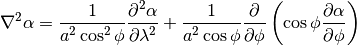
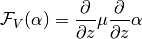
3. The Primitive Equations in General Coordinates
Ocean dynamics are described by the 3-D primitive equations for a thin
stratified fluid using the hydrostatic and Boussinesq approximations.
Before deriving the equations in general coordinates, we first present,
as a reference point, the continuous equations in spherical polar
coordinates with vertical  -coordinate. These are standard in
Bryan-Cox models (Semtner 1986; Pacanowski and Griffies 2000).
-coordinate. These are standard in
Bryan-Cox models (Semtner 1986; Pacanowski and Griffies 2000).
Momentum equations:
(1)
(2)
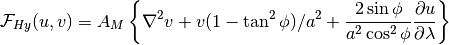
(3)¶![{\cal L}(\alpha) = \frac{1}{a\cos\phi} \left[\frac{\partial}{
\partial\lambda} (u\alpha) + \frac{\partial}{\partial\phi}
(\cos\phi v\alpha)\right] + \frac{\partial}{\partial z} (w\alpha)](../_images/math/c7889349d60f2b7ab0c621a0b7dc350125c61605.png)
(4)
(5)
(6)
(7)
Continuity equation:
(8)
Hydrostatic equation:
(9)
Equation of state:
(10)
Tracer transport:
(11)
(12)
(13)
where  ,
,  ,
,  are longitude,
latitude, and depth relative to mean sea level
are longitude,
latitude, and depth relative to mean sea level  ;
;  is
the acceleration due to gravity,
is
the acceleration due to gravity,  is the
Coriolis parameter, and
is the
Coriolis parameter, and  is the background density of
seawater. The prognostic variables in these equations are the eastward
and northward velocity components (
is the background density of
seawater. The prognostic variables in these equations are the eastward
and northward velocity components ( ,
,  ), the vertical
velocity
), the vertical
velocity  , the pressure
  , the density
  ,
and the potential temperature
,
and the potential temperature  and salinity
  . In
(11)
. In
(11)  represents ,
or a passive tracer. The pressure dependence of the equation
of state is usually approximated to be a function of depth only (see
Sec. Equation of State).
represents ,
or a passive tracer. The pressure dependence of the equation
of state is usually approximated to be a function of depth only (see
Sec. Equation of State).  and
and  are the coefficients (here
assumed to be spatially constant) for horizontal diffusion and
viscosity, respectively, and
are the coefficients (here
assumed to be spatially constant) for horizontal diffusion and
viscosity, respectively, and  and
and  are the
corresponding vertical mixing coefficients which typically depend on the
local state and mixing parameterization (see Chapter ref:`ch-subgrid). The
third terms on the left-hand side in (1) and
(2) are metric terms due to the convective derivatives in
are the
corresponding vertical mixing coefficients which typically depend on the
local state and mixing parameterization (see Chapter ref:`ch-subgrid). The
third terms on the left-hand side in (1) and
(2) are metric terms due to the convective derivatives in
 acting on the unit vectors in the ,
directions, and the second and third terms in brackets in
(4) and (5) ensure that no
stresses are generated due to solid-body rotation (Williams 1972). The
forcing terms due to wind stress and heat and fresh water fluxes are
applied as surface boundary conditions to the friction and diffusive
terms
acting on the unit vectors in the ,
directions, and the second and third terms in brackets in
(4) and (5) ensure that no
stresses are generated due to solid-body rotation (Williams 1972). The
forcing terms due to wind stress and heat and fresh water fluxes are
applied as surface boundary conditions to the friction and diffusive
terms  and
and  . The bottom and lateral
boundary conditions applied in POP (and in most other Bryan-Cox models)
are no-flux for tracers (zero tracer gradient normal to boundaries) and
no-slip for velocities (both components of velocity zero on bottom and
lateral boundaries).
. The bottom and lateral
boundary conditions applied in POP (and in most other Bryan-Cox models)
are no-flux for tracers (zero tracer gradient normal to boundaries) and
no-slip for velocities (both components of velocity zero on bottom and
lateral boundaries).
To derive the primitive equations in general coordinates, consider the
transformation from Cartesian coordinates ( ,
,  ,
,
 with origin at the center of the Earth) to general
horizontal coordinates (
with origin at the center of the Earth) to general
horizontal coordinates ( ,
,  , ), where
and are arbitrary curvilinear coordinates in the
horizontal directions, and is again the vertical
coordinate normal to the surface of the sphere. The actual distances
along the curvilinear coordinates are denoted
, ), where
and are arbitrary curvilinear coordinates in the
horizontal directions, and is again the vertical
coordinate normal to the surface of the sphere. The actual distances
along the curvilinear coordinates are denoted  and
and  ,
which typically lie along the circumpolar (longitude-like) and azimuthal
(latitude-like) coordinate lines, respectively, on dipole grids with two
arbitrarily located poles (see Sec. Global Orthogonal Grids). The differential
length element
,
which typically lie along the circumpolar (longitude-like) and azimuthal
(latitude-like) coordinate lines, respectively, on dipole grids with two
arbitrarily located poles (see Sec. Global Orthogonal Grids). The differential
length element  is given by
(14)
(15)
(where  and repeated indices are summed). The metric
coefficients
and repeated indices are summed). The metric
coefficients  depend on the local curvature of the
coordinates. Differential lengths in the direction are assumed
independent of and , so no metric coefficients
involving appear. Further restricting ourselves to orthogonal
grids, the cross terms vanish, and we have
depend on the local curvature of the
coordinates. Differential lengths in the direction are assumed
independent of and , so no metric coefficients
involving appear. Further restricting ourselves to orthogonal
grids, the cross terms vanish, and we have
(16)
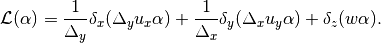
For the purpose of constructing horizontal finite-difference operators corresponding to the various terms in the primitive equations, define:

(17)
where  and
and  can be interpreted as
either infinitesimal or finite differences and their associated
derivatives. Formulas for the basic horizontal operators (gradient,
divergence, curl) can be found in standard textbooks (Arfken 1970). The
gradient is
can be interpreted as
either infinitesimal or finite differences and their associated
derivatives. Formulas for the basic horizontal operators (gradient,
divergence, curl) can be found in standard textbooks (Arfken 1970). The
gradient is
(18)
where  and
and  are unit vectors in
the
are unit vectors in
the  directions. The horizontal divergence is:
(19)
where  and
and  are the velocity components along the
and directions. The advection operator
(3) is similar:
are the velocity components along the
and directions. The advection operator
(3) is similar:
(20)
The vertical component of the curl operator is
(21)
Laplacian-type operators, which appear in the viscous and diffusive terms, have the form
(22)
where  is an arbitrary scalar function of and
. Note that these operators have been expressed in terms of the
differences and derivatives and , and
hence there is no explicit dependence on the new coordinates
is an arbitrary scalar function of and
. Note that these operators have been expressed in terms of the
differences and derivatives and , and
hence there is no explicit dependence on the new coordinates  or the metric coefficients
  . In the discrete operators the
same is true: it is not necessary to have an analytic transformation
with metric coefficients describing the new coordinate system, it is
only necessary to know the location of the discrete grid points and the
distances between neighboring grid points along the coordinate
directions.
. In the discrete operators the
same is true: it is not necessary to have an analytic transformation
with metric coefficients describing the new coordinate system, it is
only necessary to know the location of the discrete grid points and the
distances between neighboring grid points along the coordinate
directions.
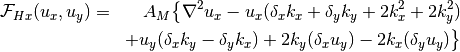
The other horizontal finite difference operators appearing in the primitive equations can also be derived in general coordinates. The Coriolis terms are simply given by
(23)
The metric momentum advection terms corresponding to the third terms on the left in (1) and (2) are given by Haltiner and Williams (1980) (p. 442):
(24)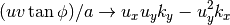
(25)
(26)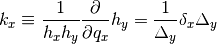
(27)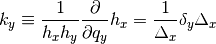
Note that these revert to the standard forms (left of arrows) in
spherical polar coordinates, where  ,
,
 ,
,  and
and  . The metric terms
in the viscous operators (second and third terms on the right in
(4) and (5) require a more
careful treatment. These terms were derived by Williams (1972) in
spherical coordinates, by applying the thin-shell approximation
(
. The metric terms
in the viscous operators (second and third terms on the right in
(4) and (5) require a more
careful treatment. These terms were derived by Williams (1972) in
spherical coordinates, by applying the thin-shell approximation
( ) to the viscous terms expressed as the divergence of a
stress tensor whose components are linearly proportional to the
components of the rate-of-strain tensor. This form is transversely
isotropic and ensures that for solid rotation the fluid is stress-free.
The general coordinate versions of these terms are derived in Smith,
Kortas, and Meltz (1995). The results are
) to the viscous terms expressed as the divergence of a
stress tensor whose components are linearly proportional to the
components of the rate-of-strain tensor. This form is transversely
isotropic and ensures that for solid rotation the fluid is stress-free.
The general coordinate versions of these terms are derived in Smith,
Kortas, and Meltz (1995). The results are
(28)
The formula for  is the same with
and interchanged everywhere on the r.h.s. It is
straightforward to show that these also reduce to the correct form in
the spherical polar limit (4),
(5). The above forms assume a spatially constant
viscosity . More terms appear if is allowed to
vary spatially. Wajsowicz (1993) derives the extra terms for spherical
polar coordinates. In general orthogonal coordinates they take the form:
is the same with
and interchanged everywhere on the r.h.s. It is
straightforward to show that these also reduce to the correct form in
the spherical polar limit (4),
(5). The above forms assume a spatially constant
viscosity . More terms appear if is allowed to
vary spatially. Wajsowicz (1993) derives the extra terms for spherical
polar coordinates. In general orthogonal coordinates they take the form:
(29)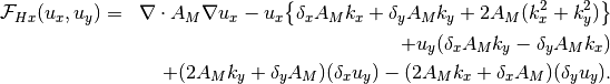
The formula for is again the same with
and interchanged everywhere.
The general coordinate forms of the anisotropic and biharmonic viscous operators are given in Sec. Horizontal Viscosity below, and the Gent-McWilliams and biharmonic forms of the horizontal diffusion terms are given in Sec. ”ref:sec-horiz-diff.
4. Spatial Discretization
4.1. Discrete Horizontal and Vertical Grids
The placement of model variables on the horizontal B-grid is illustrated
in Figure3.1. The solid lines enclose a “T-cell” and the
hatched lines enclose a “U-cell”. Scalars ( ) are
located at “T-points” (circles) at the centers of T-cells, and
horizontal vectors (
) are
located at “T-points” (circles) at the centers of T-cells, and
horizontal vectors ( ) are located at “U-points”
(diamonds) at the corners of T-cells. The indexing for points
(
) are located at “U-points”
(diamonds) at the corners of T-cells. The indexing for points
( ) in the logically-rectangular 2-D horizontal grid is such
that
) in the logically-rectangular 2-D horizontal grid is such
that  increases in the direction (eastward for
spherical polar coordinates), and
increases in the direction (eastward for
spherical polar coordinates), and  increases in the
direction (northward for spherical polar coordinates). A U-point with
logical indices () lies to the upper right
(
increases in the
direction (northward for spherical polar coordinates). A U-point with
logical indices () lies to the upper right
( northeast) of the T-point with the same indices
(). The index for the vertical dimension
northeast) of the T-point with the same indices
(). The index for the vertical dimension  increases
with depth, although the vertical coordinate , measured from
the mean surface level
increases
with depth, although the vertical coordinate , measured from
the mean surface level  , decreases with depth.
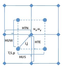
Figure 3.1: The staggered horizontal B-grid. The -coordinate grid index increases to the right (generally eastward),
and the -coordinate index increases upward (generally northward). Solid lines enclose a T-cell, hatched lines a U-cell.
The quantities labeled HTN, HTE, HUW, HUS, as well as the model prognostic variables (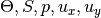 ) at the locations
shown all have grid indices ().
) at the locations
shown all have grid indices ().
When the horizontal grid is generated, the latitude and longitude of each U-point and the distances HTN and HTE (see Figure3.1 ) along the coordinates between adjacent U-points are first constructed. Then the latitude and longitude of T-points are computed as the straight average of the latitude and longitude of the four surrounding U-points, and the along-coordinate distances HUW (HUS) between adjacent T-points are computed as the straight average of the four surrounding values of HTE (HTN). Thus T-points are located exactly in the middle of the T-cell, but because the grid spacing in either direction may be non-uniform, the U-points are not located exactly in the middle of the U-cell.
In addition to the grid spacings HTN, HTE, HUS, HUW, several other lengths and areas are also used in the code. These are defined as follows (see Figure3.1 ):
(30)¶![\begin{aligned}
\mathrm{DXU}_{i,j}&=&[\mathrm{HTN}_{i,j}+\mathrm{HTN}_{i+1,j}]/2
\nonumber \\
\mathrm{DYU}_{i,j}&=&[\mathrm{HTE}_{i,j}+\mathrm{HTE}_{i,j+1}]/2
\nonumber \\
\mathrm{DXT}_{i,j}&=&[\mathrm{HTN}_{i,j}+\mathrm{HTN}_{i,j-1}]/2
\nonumber \\
\mathrm{DYT}_{i,j}&=&[\mathrm{HTE}_{i,j}+\mathrm{HTE}_{i-1,j}]/2
\nonumber \\
\mathrm{UAREA}_{i,j}&=&\mathrm{DXU}_{i,j}\mathrm{DYU}_{i,j}
\nonumber \\
\mathrm{TAREA}_{i,j}&=&\mathrm{DXT}_{i,j}\mathrm{DYT}_{i,j}
\end{aligned}](../_images/math/05098129f8afba951fe534c66516803039eb8ec8.png)
DXU and DYU are the grid lengths centered on U-points, and DXT and DYT are centered on T-points. TAREA and UAREA are the horizontal areas of T-cells and U-cells, respectively.
The construction of the semi-analytic dipole and tripole grids commonly
used in POP is described in detail in Smith, Kortas, and Meltz (1995),
and is briefly reviewed in Chapter Grids. These grids are based on
an underlying orthogonal curvilinear coordinate system with the one or
two singularities in the northern hemisphere displaced into land masses
(typically North America, Asia, or Greenland). The equator is usually
retained as a grid line and the southern hemisphere is a standard
spherical polar grid with the southern grid pole located at the true
South Pole. These grids are topologically equivalent to a cylinder
(periodic in but not in ), and therefore can be
mapped onto a logically-rectangular 2-D array () which is
cyclic in . Tripole grids require additional communication
along the northern boundary of the grid in order to “sew up” the grid
along the line between the two northern grid poles. The grids are
constructed off line and a file is generated which contains the
following 2-D fields: ULAT,ULONG,HTN,HTE,HUS,HUW,ANGLE, where
 and
and  are the
true latitude and longitude of U-points, and
are the
true latitude and longitude of U-points, and
 is the angle between the
-direction and true east at the U-point ().
is the angle between the
-direction and true east at the U-point ().
In addition to constructing the grids, the fields ULAT, ULONG and ANGLE
are used to interpolate the wind stress fields from a latitude-longitude
grid to the model grid if needed. ULAT is also used to compute the
Coriolis parameter  at each model grid point.
Figure 3.2 is a diagram of the full three-dimensional T-cell,
showing the location of the vertical velocities and
 , which advect tracers and momentum, respectively. Note that
the vertical velocities are located in the middle of the top
and bottom faces of the T-cell, while the horizontal velocities are
located at the midpoints of the vertical edges.
, which advect tracers and momentum, respectively. Note that
the vertical velocities are located in the middle of the top
and bottom faces of the T-cell, while the horizontal velocities are
located at the midpoints of the vertical edges.
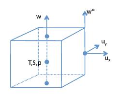
Figure 3.2: The 3-D T-cell, showing the location of the vertical velocity in T-columns and U-columns.
Since POP is a -level model, the depth of each point
( ) is independent of its horizontal location (unless
partial bottom cells are used, see Sec. Partial Bottom Cells). The vertical
discretization is illustrated in Figure3.3. The discrete
index increases from the surface (
) is independent of its horizontal location (unless
partial bottom cells are used, see Sec. Partial Bottom Cells). The vertical
discretization is illustrated in Figure3.3. The discrete
index increases from the surface ( ) to the deepest
level (
) to the deepest
level ( ). The thickness of cells at level is
 . T-points are located exactly in the middle of each level,
but because the vertical grid may be non-uniform
(
. T-points are located exactly in the middle of each level,
but because the vertical grid may be non-uniform
( ), the interfaces where the vertical velocities
lie are not exactly halfway between the T-points. The vertical
distances between T-points
), the interfaces where the vertical velocities
lie are not exactly halfway between the T-points. The vertical
distances between T-points  are just the average
 , except at the surface where
 . The depth of a T-point at level is
 , and
, and  is the depth of the bottom of cells at
level . Note that while the coordinate is positive
upward, and are positive depths. Vertical
profiles of are usually generated offline and read in by
the code, but there is an option for generating this profile internally.
Usually is small in the upper ocean and increases with
depth according to a smooth analytic function describing the thickness
as a function of depth. This is necessary in order to maintain the
formal second-order accuracy of the vertical discretization; if the
vertical spacing changes suddenly the scheme reverts to first order
accuracy (Smith, Kortas, and Meltz 1995).
is the depth of the bottom of cells at
level . Note that while the coordinate is positive
upward, and are positive depths. Vertical
profiles of are usually generated offline and read in by
the code, but there is an option for generating this profile internally.
Usually is small in the upper ocean and increases with
depth according to a smooth analytic function describing the thickness
as a function of depth. This is necessary in order to maintain the
formal second-order accuracy of the vertical discretization; if the
vertical spacing changes suddenly the scheme reverts to first order
accuracy (Smith, Kortas, and Meltz 1995).
Figure 3.3: The vertical grid.
The topography is defined in the T-cells, which are completely filled
with either land or ocean (except when optional partial bottom cells are
used; see Sec. Partial Bottom Cells). Thus U-points lie exactly on the lateral
boundaries between land and ocean, and points lie exactly on
the ocean floor. These boundary velocities are by default set to zero
for no-slip boundary conditions, though can be modified by
parameterizations like the overflow parameterization
(Sec. Overflow Parameterization). Vertical velocities along the rims in
the stair-step topography may also be nonzero (see the discussion of
velocity boundary conditions in Sec. Momentum Advection). The
topography is determined by the 2-D integer field
 which gives the number of open ocean points
in each vertical column of T-cells. The KMT field is usually generated
offline and read in from a file in the code. Thus
which gives the number of open ocean points
in each vertical column of T-cells. The KMT field is usually generated
offline and read in from a file in the code. Thus
 , and
, and  indicates a
surface land point. In some situations the ocean depth in a column of
U-points is needed, and this is defined by the field
indicates a
surface land point. In some situations the ocean depth in a column of
U-points is needed, and this is defined by the field
 , which is just the minimum of the four
surrounding values of KMT:
, which is just the minimum of the four
surrounding values of KMT:

The depths of columns of ocean T-points and U-points are given, respectively, by:
(31)
With partial bottom cells the depth of the deepest ocean cell in each column has variable thickness, and the above formulas are modified accordingly (see Sec. Partial Bottom Cells).
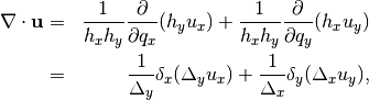
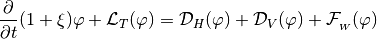
4.2. Finite-difference operators
The exact finite-difference versions of the differential operators can be easily derived for the various types of staggered horizontal grids A,B,C,D,E (Arakawa and Lamb 1977) given only the forms of the fundamental operators: divergence, gradient, and curl for that type of mesh. POP employs a B-grid (scalars at cell centers, vectors at cell corners) while some OGCM’s use a C-grid (scalars at cell centers, vector components normal to cell faces). We will use standard notation (Semtner 1986) for finite-difference derivatives and averages:
(32)¶![\begin{aligned}
\delta_x\psi &=& \left[\psi\left(x + \Delta_x/2\right) -
\psi\left(x - \Delta_x/2\right)\right]\big/\Delta_x
\\
\overline{\psi}^x &=& \left[\psi\left(x + \Delta_x/2\right) +
\psi \left(x - \Delta_x/2\right)\right]\big/2\;,
\end{aligned}](../_images/math/671c3a153632bbaab310adadb93ce27092a6f6ad.png)
with similar definitions for differences and averages in the
and directions. These formulas strictly apply for uniform grid
spacing; where, for example, if  is a tracer located at
T-points, then
is a tracer located at
T-points, then  is located on the
east face of a T-cell. For nonuniform grid spacing, the above
definitions should be interpreted such that variables lie exactly at T-
or U-cell centers and faces, as appropriate.
is located on the
east face of a T-cell. For nonuniform grid spacing, the above
definitions should be interpreted such that variables lie exactly at T-
or U-cell centers and faces, as appropriate.
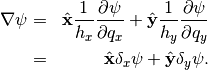
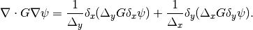
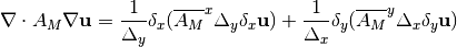
The fundamental operators on C-grids have the same form as (18) -(22). On B-grids the derivatives involve transverse averaging, and the fundamental operators are given by:
(33)¶![\begin{aligned}
\nabla\psi & = \hat{\bf x} \delta_x \overline\psi^y + \hat{\bf y} \delta_y \overline\psi^x \\
\nabla \cdot{\bf u} & = \frac{1}{\Delta_y} \delta_x \overline{\Delta_y u_x}^y + \frac{1}{\Delta_x} \delta_y \overline{\Delta_x u_y}^x \\
\hat{\bf z} \cdot \nabla \times {\bf u} & = \frac{1}{\Delta_y} \delta_x \overline{\Delta_y u_y}^y - \frac{1}{\Delta_x} \delta_y \overline{\Delta_x u_x}^x \\
\nabla\cdot G\nabla \psi & = \frac{1}{\Delta_y} \delta_x \overline{\big[\Delta_y G\delta_x \overline{\psi}^y \big]}^y
+ \frac{1}{\Delta_x} \delta_y \overline{\big[\Delta_x G\delta_y \overline{\psi}^x \big]}^x\;.
\end{aligned}](../_images/math/02870d34787d49968daa2b6fd00cb45a518012d3.png)
The gradient is located at U-points and the divergence, curl and
Laplacian are located at T-points. In the Laplacian operator
must also be defined at U-points. The factors  ,
,
 inside the difference operators
  ,
,
 are located at U-points and are given by DXU, DYU,
respectively, while the factors
are located at U-points and are given by DXU, DYU,
respectively, while the factors  ,
,  outside the difference operators, as well as similar factors in the
denominators of the difference operators ,
, are evaluated at T-points. For example, the first term
on the r.h.s. of the divergence (33) at the T-point
outside the difference operators, as well as similar factors in the
denominators of the difference operators ,
, are evaluated at T-points. For example, the first term
on the r.h.s. of the divergence (33) at the T-point  is given by
![\begin{aligned}
&&0.5[\mathrm{DYU}_{i,j}(u_x)_{i,j}
+\mathrm{DYU}_{i,j-1}(u_x)_{i,j-1} \nonumber \\
&&-\mathrm{DYU}_{i-1,j}(u_x)_{i-1,j}
-\mathrm{DYU}_{i-1,j-1}(u_x)_{i-1,j-1}]/\mathrm{TAREA}_{i,j}\end{aligned}](../_images/math/5a87c459bfb2246c4ff288724b3998d840856664.png)
In POP (and in other Bryan-Cox models which use a B-grid formulation) all viscous and diffusive terms are given in terms of an approximate C-grid discretization in order to ensure they will damp checkerboard oscillations on the scale of the grid spacing (see Secs. Horizontal Tracer Diffusion, Horizontal Tracer Diffusion, and Horizontal Viscosity).
4.3. Discrete Tracer Transport Equations
The discrete tracer transport equations are:
(34)
where  is the advection operator in T-cells, and
 , are the horizontal and vertical
diffusion operators, respectively. The factor
, are the horizontal and vertical
diffusion operators, respectively. The factor  is
associated with the change in volume of the surface layer due to
undulations of the free surface, and
is
associated with the change in volume of the surface layer due to
undulations of the free surface, and  is
the change in tracer concentration associated with the freshwater flux.
is
the change in tracer concentration associated with the freshwater flux.
 and are given by
(35)
(36)
where  is the Kronecker delta, equal to 1 for
and zero otherwise.
is the Kronecker delta, equal to 1 for
and zero otherwise.  is the displacement of the
free surface relative to ,
is the displacement of the
free surface relative to ,  is the
freshwater flux per unit area associated with a specific source (labeled
is the
freshwater flux per unit area associated with a specific source (labeled
 ) of freshwater. Thus,
 is the total freshwater flux per unit area associated with precipitation
 , evaporation
  , river runoff
  , freezing
 and melting
  of sea ice, and
 is the tracer concentration in the freshwater
associated with source . The change in volume of the surface
layer due to the freshwater flux is discussed in Sec.:ref:sec-linear-free-surface,
and the natural boundary conditions for
tracers associated with freshwater flux are discussed in
Sec. Variable-Thickness Surface Layer. The boundary conditions on tracers are no-flux
normal to bottom and lateral boundaries, unless modified by
parameterizations like the overflow parameterization (see
Sec. Overflow Parameterization).
is the tracer concentration in the freshwater
associated with source . The change in volume of the surface
layer due to the freshwater flux is discussed in Sec.:ref:sec-linear-free-surface,
and the natural boundary conditions for
tracers associated with freshwater flux are discussed in
Sec. Variable-Thickness Surface Layer. The boundary conditions on tracers are no-flux
normal to bottom and lateral boundaries, unless modified by
parameterizations like the overflow parameterization (see
Sec. Overflow Parameterization).
4.3.1. Tracer Advection
POP has multiple options for tracer advection. Here we describe a basic second-order centered advection scheme as an example of a discretization. Other advection schemes are described in Chapter Advection. In the standard second-order scheme, the advection operator is given by:
(37)
Again, and inside the difference
operator are located at U-points, and the mass fluxes
 ,
,  are
located on the lateral faces of T-cells.
are
located on the lateral faces of T-cells.  and
and  are also located on the lateral faces
of T-cells, while
are also located on the lateral faces
of T-cells, while  is located on the top and
bottom faces of T-cells. At the surface, is
set equal to zero because there is no advection of tracers across the
surface. The vertical velocity at T-points is determined from
the solution of the continuity equation
is located on the top and
bottom faces of T-cells. At the surface, is
set equal to zero because there is no advection of tracers across the
surface. The vertical velocity at T-points is determined from
the solution of the continuity equation
(38)
which is integrated in a column of T-cells downward from the top with the boundary conditions:
(39)
(40)
The boundary condition (39) is discussed in more detail in Sec.:ref:sec-linear-free-surface.
When integrating from the top down using (38) and
(39), the bottom boundary condition (40) will only be
satisfied to the extent that the solution of the elliptic system of
barotropic equations for the surface height has converged
exactly (see Sec. Barotropic Equations). In practice, this exact
convergence is not achieved, so the bottom velocity in T-columns is set
to zero to ensure no tracers are fluxed through the bottom. This amounts
to allowing a very small divergence of velocity in the bottom cell.
In versions of POP prior to 1.4.3, the volume of the surface cells is
assumed constant, and no account is taken of the change in volume of the
surface cells when the free surface height changes. Thus  and
and  in (34), (35) and (36), and the
freshwater flux is approximated as a virtual salinity flux and imposed
as a boundary condition on the vertical diffusion operator. In addition,
the tracers are advected through the surface in this formulation using
(37) with the vertical velocity given by (39) and
in (34), (35) and (36), and the
freshwater flux is approximated as a virtual salinity flux and imposed
as a boundary condition on the vertical diffusion operator. In addition,
the tracers are advected through the surface in this formulation using
(37) with the vertical velocity given by (39) and
 at the surface. One problem
with this approximation is that the advective flux of tracers through
the surface is not zero in global average. The globally integrated
vertical mass flux vanishes, but the integrated tracer flux does not. In
practice, we have found that the residual surface tracer fluxes
associated with this are usually small, but in some situations they may
be non-negligible. (Note: the global mean residual surface tracer fluxes
are standard diagnostic model output in the earlier versions of POP
without the variable thickness surface layer.) Because the residual
surface flux is nonzero, the global mean tracers are not conserved. In
POP version 1.4.3, the surface layer is based on (34), (35)
and (36), and global mean tracers (in particular total salt) are
conserved exactly. The variable-thickness surface layer is detailed in
Sec. Variable-Thickness Surface Layer.
at the surface. One problem
with this approximation is that the advective flux of tracers through
the surface is not zero in global average. The globally integrated
vertical mass flux vanishes, but the integrated tracer flux does not. In
practice, we have found that the residual surface tracer fluxes
associated with this are usually small, but in some situations they may
be non-negligible. (Note: the global mean residual surface tracer fluxes
are standard diagnostic model output in the earlier versions of POP
without the variable thickness surface layer.) Because the residual
surface flux is nonzero, the global mean tracers are not conserved. In
POP version 1.4.3, the surface layer is based on (34), (35)
and (36), and global mean tracers (in particular total salt) are
conserved exactly. The variable-thickness surface layer is detailed in
Sec. Variable-Thickness Surface Layer.
4.3.2. Horizontal Tracer Diffusion
POP has three options for horizontal tracer diffusion: 1) horizontal Laplacian diffusion, 2) horizontal biharmonic diffusion, 3) the Gent-McWilliams parameterization, which includes along-isopycnal tracer diffusion and tracer advection with an additional eddy-induced transport velocity. All of these are implemented for a spatially varying diffusivity. The first of these options (Laplacian diffusion) is described here, the other two options are discussed in Sec. Horizontal Tracer Diffusion. The discrete horizontal Laplacian diffusion operator is given by:
(41)
Note that no lateral averaging is involved as in (33). Thus
the Laplacian is approximated as a five-point stencil as would be used
on a C-grid. The factors , inside the
difference operator are given by HTN, HTE, respectively (see
Figure3.1 ), and , defined at T-points, is
averaged across the T-cell faces. As mentioned above, all the horizontal
diffusive operators in POP that would normally involve nine-point
operators (including the GM parameterization and the horizontal friction
operators), are approximated by five-point C-grid operators in order to
ensure that they damp checkerboard noise on the grid scale. B-grid
Laplacian-type operators like (33) have a checkerboard null
space, i.e., they yield zero when applied to a  checkerboard
field, and thus cannot damp noise of this character (see
Sec. Nullspace Removal). The only Laplacian-type operator which uses a
B-grid discretization is the elliptic operator in the implicit
barotropic system. There the B-grid discretization is required in order
to maintain energetic consistency (Smith, Dukowicz, and Malone 1992;
Dukowicz, Smith, and Malone 1993), see also
Secs. Energetic Consistency and Barotropic Equations). The
boundary conditions on the diffusive operator (41) are that
tracer gradients
checkerboard
field, and thus cannot damp noise of this character (see
Sec. Nullspace Removal). The only Laplacian-type operator which uses a
B-grid discretization is the elliptic operator in the implicit
barotropic system. There the B-grid discretization is required in order
to maintain energetic consistency (Smith, Dukowicz, and Malone 1992;
Dukowicz, Smith, and Malone 1993), see also
Secs. Energetic Consistency and Barotropic Equations). The
boundary conditions on the diffusive operator (41) are that
tracer gradients  ,
,  are
zero normal to lateral boundaries.
are
zero normal to lateral boundaries.
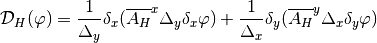
4.3.3. Vertical Tracer Diffusion
The spatial discretization of the vertical diffusion operator is given by:
(42)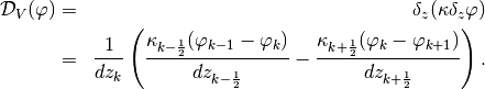
where  is a tracer at level , and
 ,
,  are
evaluated on the top and bottom faces, respectively, of the T-cell at
level , and
are
evaluated on the top and bottom faces, respectively, of the T-cell at
level , and  ,
,
 . The boundary conditions at the top
and bottom of the column are
. The boundary conditions at the top
and bottom of the column are
(43)
where  is the surface flux of tracer
(e.g., heat flux for temperature and equivalent salt flux associated
with freshwater flux for salinity). The modifications to this
discretization when partial bottom cells are used is described in
Sec. Partial Bottom Cells. The diffusive term may either be evaluated explicitly or
implicitly. The implicit treatment is described in Sec. Implicit Vertical Diffusion.
With explicit mixing, a convective adjustment routine may also be used
to more efficiently mix tracers when the column is unstable (see
Sec. Convection). Various subgrid-scale parameterizations for the
vertical diffusivity are discussed in Sec. Vertical Mixing.
is the surface flux of tracer
(e.g., heat flux for temperature and equivalent salt flux associated
with freshwater flux for salinity). The modifications to this
discretization when partial bottom cells are used is described in
Sec. Partial Bottom Cells. The diffusive term may either be evaluated explicitly or
implicitly. The implicit treatment is described in Sec. Implicit Vertical Diffusion.
With explicit mixing, a convective adjustment routine may also be used
to more efficiently mix tracers when the column is unstable (see
Sec. Convection). Various subgrid-scale parameterizations for the
vertical diffusivity are discussed in Sec. Vertical Mixing.
4.4. Discrete Momentum Equations.
The momentum equations discretized on the B-grid are given by:
(44)
(45)
In these equations no account has been taken of the change in volume of
the surface layer due to undulations of the free surface. Therefore, no
terms involving appear as in the tracer transport equation
(34). The justification for this is that the global mean
momentum, unlike the global mean tracers, is not conserved in the
absence of forcing, so there is less motivation to correct for momentum
nonconservation due to surface height fluctuations. Furthermore, the
error introduced is typically small compared to the uncertainty in the
applied wind stress.
Note: Currently the code is in cgs units and it is assumed that
 g cm
g cm , so it never explicitly
appears. If the Boussinesq correction (Sec. Boussinesq Correction) is used,
then this factor is already taken into account, because the factor
, so it never explicitly
appears. If the Boussinesq correction (Sec. Boussinesq Correction) is used,
then this factor is already taken into account, because the factor
 in (229) is normalized such that the pressure gradient
should be divided by
in (229) is normalized such that the pressure gradient
should be divided by  .
.
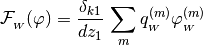
4.4.1. Momentum Advection
The nonlinear momentum advection term is discretized as:
(46)¶![{\cal L}_{U}(\alpha) = \frac{1}{\Delta_y} \delta_x
\big[\overline{(\overline{\Delta_y u_x}^y)}^{xy}
\overline{\alpha}^x\big]
+ \frac{1}{\Delta_x} \delta_y
\big[\overline{(\overline{\Delta_x u_y}^x)}^{xy}
\overline{\alpha}^y\big]
+ \delta_z (w^U\overline{\alpha}^z)\;.](../_images/math/42c112a2618b175e55d409f45ad1e4a2919b4b41.png)
This is a second-order centered advection scheme and is currently the
only option available in POP for momentum advection. It has the property
that global mean kinetic energy is conserved by advection. Momentum is
conserved in the interior by advection, but not on the boundaries (see
Sec. Energetic Consistency on energetic consistency). The mass
fluxes in the operator include an extra average in both horizontal
directions, denoted  . Both the horizontal
and vertical mass fluxes in a U-cell are the average of the four
surrounding T-cell mass fluxes. This is illustrated in
Figure3.4 for the mass flux in the -direction. As a
consequence, the vertical velocity in a U-cell is exactly the
area-weighted average of the four surrounding T-cell vertical velocities
. This averaging is necessary in order to maintain the
energetic balance between the global mean work done by the pressure
gradient and the change in gravitational potential energy (Smith,
Dukowicz, and Malone 1992), see also Sec. Energetic Consistency on
energetic consistency. An additional advantage of this flux averaging in
U-cells is that it substantially reduces noise in the vertical velocity
field compared to other approaches (Webb 1995). At the bottom of a
column of ocean U-cells is not necessarily zero, because it
is the weighted average of the surrounding ’s, some of which
may be nonzero if it is a “rim” point where
. Both the horizontal
and vertical mass fluxes in a U-cell are the average of the four
surrounding T-cell mass fluxes. This is illustrated in
Figure3.4 for the mass flux in the -direction. As a
consequence, the vertical velocity in a U-cell is exactly the
area-weighted average of the four surrounding T-cell vertical velocities
. This averaging is necessary in order to maintain the
energetic balance between the global mean work done by the pressure
gradient and the change in gravitational potential energy (Smith,
Dukowicz, and Malone 1992), see also Sec. Energetic Consistency on
energetic consistency. An additional advantage of this flux averaging in
U-cells is that it substantially reduces noise in the vertical velocity
field compared to other approaches (Webb 1995). At the bottom of a
column of ocean U-cells is not necessarily zero, because it
is the weighted average of the surrounding ’s, some of which
may be nonzero if it is a “rim” point where  but
at least one of the surrounding T-points has
but
at least one of the surrounding T-points has  . It
can be shown that the value of at these points approximates
the boundary condition for tangential flow along the sloping bottom
. It
can be shown that the value of at these points approximates
the boundary condition for tangential flow along the sloping bottom
 (Semtner 1986). Momentum is advected
through the surface using the vertical velocity (39) averaged to
U-points and with
(Semtner 1986). Momentum is advected
through the surface using the vertical velocity (39) averaged to
U-points and with  (where
 or ) in (46).
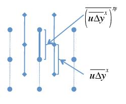
Figure 3.4: Advective mass fluxes through lateral faces of T-cells (narrow solid lines) and U-cells (thick solid line). U-cell fluxes are the average of the four surrounding T-cell fluxes. A similar averaging applies to the vertical fluxes.
4.4.2. Metric Terms
The metric terms (third and fourth terms on the l.h.s. in (45)) are
constructed using a simple C-grid discretization of the metric factors,
as in (26) and (27). Specifically,  and
and  at
U-points are:
at
U-points are:
(47)¶![\begin{aligned}
\mathrm{KXU}_{i,j}&=&[\mathrm{HUW}_{i+1,j}-\mathrm{HUW}_{i,j}]/\mathrm{UAREA}_{i,j}
\nonumber \\
\mathrm{KYU}_{i,j}&=&[\mathrm{HUS}_{i,j+1}-\mathrm{HUS}_{i,j}]/\mathrm{UAREA}_{i,j}
\end{aligned}](../_images/math/15fc747e4bae9e0ca1ccfbe01e771b21e1b7b1fc.png)
4.4.3. Horizontal Friction
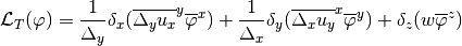
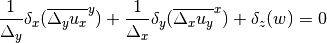
Several options for horizontal friction are available in the code. In this section a simple spatial discretization of the Laplacian-type formulation with a spatially varying viscous coefficient as given by (29) is presented. The biharmonic friction operator obtained by applying (28) twice is described in Sec. Biharmonic Horizontal Viscosity. More sophisticated formulations of the viscosity based on a functional discretization of the friction operator formulated as the divergence of a viscous stress that is linearly related to the components of the strain-rate tensor are described in Sections Anisotropic Horizontal Viscosity and Smagorinsky Nonlinear Viscous Coefficients. These include an anisotropic formulation of the viscosity and the use of Smagorinksy-type nonlinear viscous coefficients.
The Laplacian horizontal friction terms (28) and (29) are constructed from a C-grid discretization of both the Laplacian and the metric terms. The discrete Laplacian terms are given by:
(48)
where , defined at U-points, is averaged across cell faces
inside the divergence. Terms proportional to and
in (28) and (29) are evaluated using
(47). Terms involving derivatives of and
are evaluated with , defined at T-points and
averaged along U-cell faces. For example, the term
 is evaluated as:
![\begin{aligned}
&&\delta_x \overline{A_M}^x\overline{k_x}^y =
\nonumber \\
&&0.25\{[(A_M)_{i+1,j}+(A_M)_{i,j}][\mathrm{KXT}_{i+1,j+1}+\mathrm{KXT}_{i+1,j}]
\nonumber \\
&&-[(A_M)_{i,j}+(A_M)_{i-1,j}][\mathrm{KXT}_{i,j+1}+\mathrm{KXT}_{i,j}]\}
/\mathrm{DXU}_{i,j}\end{aligned}](../_images/math/72752dc9cc3a856f897ba6dd747e2886beecf8dd.png)
where is averaged across the U-cell faces, and ,
at T-points are given by
(49)¶![\begin{aligned}
\mathrm{KXT}_{i,j}&=&[\mathrm{HTE}_{i,j}-\mathrm{HTE}_{i-1,j}]/\mathrm{TAREA}_{i,j}
\nonumber \\
\mathrm{KYT}_{i,j}&=&[\mathrm{HTN}_{i,j}-\mathrm{HTN}_{i,j-1}]/\mathrm{TAREA}_{i,j}
\end{aligned}](../_images/math/b230d8136c64647c2c9a96c4e3fdd5a3afce87c6.png)
Finally, in those terms in (28),:eq:horiz-fric.2 that involve
single derivatives of the velocities or viscosities (e.g.
 or,
or,  ) the derivatives are
evaluated as differences across the cell without using the central
value. For example, at point () is
evaluated as:
) the derivatives are
evaluated as differences across the cell without using the central
value. For example, at point () is
evaluated as:
![\begin{aligned}
[(u_y)_{i+1,j}-(u_y)_{i-1,j}]/[\mathrm{HTN}_{i,j}+\mathrm{HTN}_{i+1,j}]\end{aligned}](../_images/math/11164967d8c29a4ff325ef577d13d341f0b4ebe4.png)
The no-slip boundary conditions are implemented by simply setting
 on all lateral boundary points. Modifications to
the operator when partial bottom cells are used are described in
Sec. Partial Bottom Cells.
on all lateral boundary points. Modifications to
the operator when partial bottom cells are used are described in
Sec. Partial Bottom Cells.
4.4.4. Vertical Friction
The spatial discretization of the vertical friction terms is essentially
identical to that of the vertical diffusion described in
Sec. Vertical Tracer Diffusion. The spatial discretization of both
 and
and  is identical to
(42) with replaced by the vertical viscosity
and replaced by one of the velocity
components or . Modifications for partial bottom
cells are discussed in Sec. Partial Bottom Cells. The boundary conditions at the
top and bottom of the column of U-points are
is identical to
(42) with replaced by the vertical viscosity
and replaced by one of the velocity
components or . Modifications for partial bottom
cells are discussed in Sec. Partial Bottom Cells. The boundary conditions at the
top and bottom of the column of U-points are
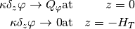
(50)
where  are the components of the surface wind
stress along the coordinate directions, and a quadratic drag term is
applied at the bottom of the column. The dimensionless constant
are the components of the surface wind
stress along the coordinate directions, and a quadratic drag term is
applied at the bottom of the column. The dimensionless constant
 is typically chosen to be of order
  . The
semi-implicit treatment of these terms is described in
Sec. Semi-Implicit Treatment of Coriolis and Vertical Friction Terms. Various subgrid-scale parameterizations for the
vertical viscosity are described in Sec. Vertical Mixing.
. The
semi-implicit treatment of these terms is described in
Sec. Semi-Implicit Treatment of Coriolis and Vertical Friction Terms. Various subgrid-scale parameterizations for the
vertical viscosity are described in Sec. Vertical Mixing.
4.5. Energetic Consistency
The energetic balances in the free-surface formulation are described in detail in Dukowicz and Smith (1994). However, this reference predates the implementation of a variable-surface thickness layer (Sec. Variable-Thickness Surface Layer) and partial bottom cells (Sec. Partial Bottom Cells), both of which influence the energetic balances.
5. Time Discretization
The POP model uses a three-time-level second-order-accurate modified leapfrog scheme for stepping forward in time. It is modified in the sense that some terms are evaluated semi-implicitly, and of the terms that are treated explicitly, only the advection operators are actually evaluated at the central time level, as in a pure leapfrog scheme. The diffusive terms are evaluated using a forward step. The reason for this is that the centered advection scheme is unstable for forward steps, and the diffusive scheme is unstable for leapfrog steps.
5.1. Filtering Timesteps
Leapfrog schemes can develop computational noise due to the partial
decoupling of even and odd timesteps. In a pure leapfrog scheme they are
completely decoupled and the solutions on the even and odd steps can
evolve independently, leading to  oscillations in time.
There are several methods to damp the leapfrog computational mode, two
of which are currently implemented in POP.
oscillations in time.
There are several methods to damp the leapfrog computational mode, two
of which are currently implemented in POP.
One is to occasionally take a forward step or an Euler forward-backward step, sometimes called a Matsuno timestep (Haltiner and Williams 1980). The Matsuno step is a forward predictor step followed by a “backward” step which is essentially a repeat of the forward step but using the predicted prognostic variables from the first pass to evaluate all terms except the time-tendency term (see Sec. Tracer Transport Equations). The Matsuno step is more expensive than a forward step, but it is stable for advection.
The other method is to occasionally perform an averaging of the solution at three successive time levels to the two intermediate times, back up half a timestep and proceed. The later procedure is referred to as an “averaging timestep” (Dukowicz and Smith 1994) and is the recommended method for eliminating the leapfrog computational mode. The leapfrog scheme generates two different “trajectories” of the solution, one corresponding to even and one to odd steps. The advantage of the averaging step is that it places the solution on the average trajectory, whereas the forward and Matsuno steps select only one trajectory, corresponding to either the even or the odd solution. Experience has shown that some model configurations are not stable using Matsuno filtering timesteps, and this is especially true with the variable-thickness surface layer (Sec. Variable-Thickness Surface Layer).
On the very first time step of a spinup from rest a forward step is taken to avoid immediately exciting a leapfrog computational mode (this feature is hardwired into the code). In the presentation below, the time discretization of various terms will first be presented for a regular leapfrog step, then the discretization for the forward and backward steps will be given.
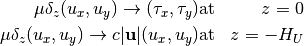
5.2. Tracer Transport Equations
Labeling the three time levels on a given step as  ,
,
 , and
, and  , the tracer transport equation (34)
is discretized in time as follows:
, the tracer transport equation (34)
is discretized in time as follows:
(51)¶![(1+\xi^{n+1})\varphi^{n+1}-(1+\xi^{n-1})\varphi^{n-1} = \\
\tau [- {\cal L}^{(n)}_T(\varphi^n) + {\cal D}_H(\varphi^{n-1})
+{\cal D}_V(\overline{\varphi}^{\lambda})
+ {\cal F}^n_{_W}]](../_images/math/3e7c12411c867461cbceb0d021d08a5278038b39.png)
where  is the timestep and
  .
.
 is given by (36) with
  and
evaluated at time , and
and
evaluated at time , and  is given
by (35) with evaluated at time . The superscript
is given
by (35) with evaluated at time . The superscript
 on the advection operator indicates that the advective mass
fluxes are evaluated using the time velocities. The vertical
diffusion term may be evaluated either explicitly or semi-implicitly. In
the explicit case
on the advection operator indicates that the advective mass
fluxes are evaluated using the time velocities. The vertical
diffusion term may be evaluated either explicitly or semi-implicitly. In
the explicit case  . For semi-implicit diffusion
 is required for stability, and the code is
usually run with
is required for stability, and the code is
usually run with  . The surface forcing (43),
applied as a boundary condition on the vertical diffusion operator, is
evaluated at time for both explicit and semi-implicit mixing.
The modifications to the tracer transport equations with implicit
vertical mixing are described in Sec. Implicit Vertical Diffusion.
. The surface forcing (43),
applied as a boundary condition on the vertical diffusion operator, is
evaluated at time for both explicit and semi-implicit mixing.
The modifications to the tracer transport equations with implicit
vertical mixing are described in Sec. Implicit Vertical Diffusion.
With pressure averaging (see Sec. Pressure Averaging) the
potential temperature and salinity at the new time are needed to
evaluate the pressure gradient at the new time. This is required in the
baroclinic momentum equations before the barotropic equations have been
solved for the surface height at the new time. Therefore,
(51) cannot be used to predict the new tracers because
 is not yet known. Instead an approximation is made to
predict the new temperature and salinity which are then used to evaluate
the pressure gradient at the new time. After the barotropic equations
have been solved, the new potential temperature and salinity are
corrected so that they satisfy (51) exactly. The equations
for predicting and correcting the tracers at the new time are obtained
as follows. The l.h.s. of (51), which involves the unknown
surface height
is not yet known. Instead an approximation is made to
predict the new temperature and salinity which are then used to evaluate
the pressure gradient at the new time. After the barotropic equations
have been solved, the new potential temperature and salinity are
corrected so that they satisfy (51) exactly. The equations
for predicting and correcting the tracers at the new time are obtained
as follows. The l.h.s. of (51), which involves the unknown
surface height  , is approximated as:
With this approximation, the equations for predicting and correcting
and are given by:
Predictor:
(52)
Corrector:
(53)
where  is the predicted tracer at the new
time, and
is the predicted tracer at the new
time, and  represents all terms in brackets on the r.h.s. of
(51). Note that these equations are used only to predict
and correct and ; all passive tracers are
updated directly using (51).
represents all terms in brackets on the r.h.s. of
(51). Note that these equations are used only to predict
and correct and ; all passive tracers are
updated directly using (51).
The time discretization for the two-time-level forward and backward steps is given by
Forward step:
(54)¶![\begin{aligned}
(1+\xi^{*})\varphi^{*}-(1+\xi^{n})\varphi^{n} & = &
\tau [- {\cal L}^{(n)}_T(\varphi^n) + {\cal D}_H(\varphi^{n})
+{\cal D}_V(\overline{\varphi}^{\lambda})
+ {\cal F}^n_{_W}] \nonumber \\
\overline{\varphi}^{\lambda} & = &
\lambda\varphi^{*} + (1-\lambda)\varphi^{n}
\end{aligned}](../_images/math/2ad30b7d71d1a9152eff814a98a63d79274f1a20.png)
Backward step:
(55)¶![\begin{aligned}
(1+\xi^{n+1})\varphi^{n+1}-(1+\xi^{n})\varphi^{n} & = &
\tau [- {\cal L}^{(*)}_T(\varphi^*) + {\cal D}_H(\varphi^{*})
+{\cal D}_V(\overline{\varphi}^{\lambda})
+ {\cal F}^n_{_W}] \nonumber \\
\overline{\varphi}^{\lambda} & = &
\lambda\varphi^{n+1} + (1-\lambda)\varphi^{n}
\end{aligned}](../_images/math/811c2792a005bf947e4ba27bc004a7c5ba9cfd6c.png)
Here  and
and  , the predicted
tracer at the new time from the forward step, is used to evaluate the
r.h.s. in the backward step.
, the predicted
tracer at the new time from the forward step, is used to evaluate the
r.h.s. in the backward step.  is given by (35) with
 .
.  is the advection
operator evaluated using the predicted velocities from the forward step
(see Sec. Baroclinic Momentum Equations). For a forward step only,
is the advection
operator evaluated using the predicted velocities from the forward step
(see Sec. Baroclinic Momentum Equations). For a forward step only,
 . The surface forcing applied to
, as well as the freshwater tracer flux
. The surface forcing applied to
, as well as the freshwater tracer flux
 , are evaluated at time in both forward
and backward steps.
, are evaluated at time in both forward
and backward steps.
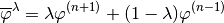
5.2.1. Tracer Acceleration
The acceleration technique of Bryan (1984) can be used to more quickly
spin up the model to a steady state by modifying the timestep for the
momentum equation, or tracers in the deep ocean. The basic method is to
modify the time step  as follows in the baroclinic and
barotropic momentum equations: (65) and
(83)
as follows in the baroclinic and
barotropic momentum equations: (65) and
(83)
and in the tracer transport equation (51)
where superscripts denote timesteps for the momentum and continuity
 , and tracers
  .
.  and
and
 are acceleration factors specified in the namelist
model input:
are acceleration factors specified in the namelist
model input:  ,
,
 , in addition to the tracer
timestep. Note that
, in addition to the tracer
timestep. Note that  is not a model input.
There are some points to make about the use of acceleration. First, a
disadvantage of depth-dependent tracer acceleration is that it leads to
non-conservative advective and diffusive fluxes when
 . For this reason, it is recommended
that profiles of be smooth functions of depth, and that
the largest vertical discontinuities in be restricted
to depths where fluxes are small enough that tracers are well conserved.
The depth-dependent tracer timestep must also be accounted for in the
convective adjustment and vertical mixing routines. These changes are
described in Secs. Convection, Tridiagonal Solver, and
Semi-Implicit Treatment of Coriolis and Vertical Friction Terms. Danabasoglu (2004) shows some detrimental effects of
the tracer non-conservation with this type of acceleration method,
including the model approaching an incorrect steady state solution.
Therefore, it is recommended that the depth-dependent tracer
acceleration not be used.
. For this reason, it is recommended
that profiles of be smooth functions of depth, and that
the largest vertical discontinuities in be restricted
to depths where fluxes are small enough that tracers are well conserved.
The depth-dependent tracer timestep must also be accounted for in the
convective adjustment and vertical mixing routines. These changes are
described in Secs. Convection, Tridiagonal Solver, and
Semi-Implicit Treatment of Coriolis and Vertical Friction Terms. Danabasoglu (2004) shows some detrimental effects of
the tracer non-conservation with this type of acceleration method,
including the model approaching an incorrect steady state solution.
Therefore, it is recommended that the depth-dependent tracer
acceleration not be used.
Second, if  , then the surface forcing for
momentum does not occur at the correct time because the model calender
and forcing fields are based on the surface tracer time step. For this
reason, if momentum acceleration,
, then the surface forcing for
momentum does not occur at the correct time because the model calender
and forcing fields are based on the surface tracer time step. For this
reason, if momentum acceleration,  , is used, then a
subsequent synchronous integration is required to get the momentum and
tracer fields back in step. This acceleration technique is recommended
by Danabasoglu (2004), who used a value of
, is used, then a
subsequent synchronous integration is required to get the momentum and
tracer fields back in step. This acceleration technique is recommended
by Danabasoglu (2004), who used a value of  . Third, if
the variable thickness surface layer option is used with virtual salt
flux boundary conditions, see Sec. Variable-Thickness Surface Layer, Danabasoglu
(2004) shows the momentum acceleration technique is stable, despite the
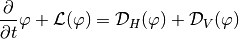
fact that the time stepping discretizations in the tracer transport and
barotropic continuity equations are inconsistent.
. Third, if
the variable thickness surface layer option is used with virtual salt
flux boundary conditions, see Sec. Variable-Thickness Surface Layer, Danabasoglu
(2004) shows the momentum acceleration technique is stable, despite the
fact that the time stepping discretizations in the tracer transport and
barotropic continuity equations are inconsistent.
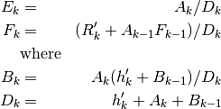
5.2.2. Implicit Vertical Diffusion
The tracer equations with implicit vertical diffusion involve the solution of a tridiagonal system in each vertical column of grid points. This is a relatively easy thing to do because the system does not involve any coupling with neighboring points in the horizontal direction. The equations solved in the code are
(56)¶![\begin{aligned}
[1+\xi^{n+1}-\lambda \tau {\sf A}(\kappa)]\Delta\varphi & = &
-(\xi^{n+1}-\xi^{n-1})\varphi^{n-1} \nonumber \\
& + & \tau [- {\cal L}_T^{(n)}(\varphi^n) +
{\cal D}_H(\varphi^{n-1}) + {\sf A}(\kappa)\varphi^{n-1}
+ {\cal F}^n_{_W}]
\nonumber \\
{\sf A}(\kappa) = \delta_z \kappa \delta_z,
&& \Delta\varphi\equiv\varphi^{n+1}-\varphi^{n-1}
\end{aligned}](../_images/math/3eda80bc07c1fb3066082dbb580748975f3f1c2c.png)
where  . For explicit diffusion ,
so the term in brackets on the right corresponds to the exact r.h.s. in
the explicit case. The system is solved for the change in tracer
. For explicit diffusion ,
so the term in brackets on the right corresponds to the exact r.h.s. in
the explicit case. The system is solved for the change in tracer
 , subject to the no-flux boundary conditions
(57)
Note that because the surface forcing and freshwater tracer fluxes are
evaluated at time , they are entirely contained in the r.h.s.
of (56) and hence are not directly imposed as a boundary
condition on the operator.
The predictor and corrector steps for updating and
with pressure averaging (Sec. Pressure Averaging) are
given by:
Predictor:
(58)¶![\begin{aligned}
[1+\xi^{n}-\lambda \tau {\sf A}(\kappa)]\Delta\varphi & = &
-2(\xi^{n}-\xi^{n-1})\varphi^n + \tau F \nonumber \\
\Delta\varphi & \equiv & \widehat{\varphi}^{n+1}-\varphi^{n-1}
\end{aligned}](../_images/math/4e243ca4d3e23224498e670206e43e941a49f3fb.png)
Corrector:
(59)¶![\begin{aligned}
[1+\xi^{n+1}-\lambda \tau {\sf A}(\kappa)]\Delta\varphi & = &
(\xi^n-\xi^{n-1})(2\varphi^n-\varphi^{n-1})
-(\xi^{n+1}-\xi^n)\widehat{\varphi}^{n+1} \nonumber \\
\Delta\varphi & \equiv & \varphi^{n+1}-\widehat{\varphi}^{n+1}
\end{aligned}](../_images/math/770f10c0bc729496697988885d1937911aa5920e.png)
where represents all terms in brackets on the right-hand side
of (56). These reduce to (52) and (53)
in the limit  . Note that both the predictor and
corrector steps involve the solution of a tridiagonal system.
. Note that both the predictor and
corrector steps involve the solution of a tridiagonal system.
In forward and backward timesteps the implicit equations have the form:
Forward step:
(60)¶![\begin{aligned}
[1+\xi^{*}-\lambda \tau {\sf A}(\kappa)]\Delta\varphi & = &
-(\xi^*-\xi^n)\varphi^n \nonumber \\
& + & \tau [- {\cal L}_{T}^{(n)}(\varphi^n)
+ {\cal D}_H(\varphi^n) + {\sf A}(\kappa)\varphi^{n}
+ {\cal F}^n_{_W}] \nonumber \\
\Delta\varphi & \equiv & \varphi^{*}-\varphi^{n}
\end{aligned}](../_images/math/fe603fae7a01bda5f5a1390dcd982e7badeedadf.png)
Backward step:
(61)¶![\begin{aligned}
[1+\xi^{n+1}-\lambda \tau {\sf A}(\kappa)]\Delta\varphi & = &
-(\xi^{n+1}-\xi^n)\varphi^n \nonumber \\
& + & \tau [- {\cal L}_{T}^{(*)}(\varphi^*)
+ {\cal D}_H(\varphi^*) + {\sf A}(\kappa)\varphi^{n}
+ {\cal F}^n_{_W}] \nonumber \\
\Delta\varphi & \equiv & \varphi^{n+1}-\varphi^{n}
\end{aligned}](../_images/math/428ef3f0692991366ffa4d6fecd8067937139b44.png)
where .
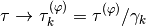
5.2.3. Tridiagonal Solver
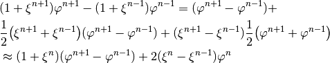
For the tridiagonal solution of (56), (58), (59), (60) or (61), a new algorithm is used (Schopf and Loughe 1995) which is more accurate and stable than traditional methods. These equations have the form:
(62)¶![(1+\xi)X_k - \lambda\frac{\tau_k}{dz_k}\big[
\frac{\kappa_{k-\frac{1}{2}}}{dz_{k-\frac{1}{2}}}
(X_{k-1} - X_{k})
- \frac{\kappa_{k+\frac{1}{2}}}{dz_{k+\frac{1}{2}}}
(X_{k} - X_{k+1})\big] = R_k](../_images/math/c115e5e37accf40b7db2af2313bba7f9b4bb8663.png)
where  at level ,
  is the
r.h.s., and a depth-dependent timestep
is the
r.h.s., and a depth-dependent timestep  (
( for leapfrog and
  for forward/backward timesteps) is used with tracer acceleration (see
Sec. Tracer Acceleration). Here
for forward/backward timesteps) is used with tracer acceleration (see
Sec. Tracer Acceleration). Here  , except in
the predictor step (58) where
, except in
the predictor step (58) where  .
(62) can be rewritten in the form of a tridiagonal system:
.
(62) can be rewritten in the form of a tridiagonal system:
(63)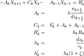
The algorithm for the solution of this system involves a loop over vertical levels to determine the coefficients:
(64)
The loop begins at with  . This is
followed by another vertical loop to determine the solution by back
substitution:
. This is
followed by another vertical loop to determine the solution by back
substitution:
This loop begins at the bottom with  when
when
 .
.
5.3. Splitting of Barotropic and Baroclinic Modes
The barotropic mode of the primitive equations supports fast gravity
waves with speeds of  200 m s:math:^{-1}. If
resolved numerically, these waves impose a severe restriction on the
model timestep. However, they have little effect on the dynamics,
especially on timescales longer than a day or so. To overcome this
severe limitation on the timestep, the barotropic mode is split off and
solved as a separate 2-D system (see Sec. Barotropic Equations).
200 m s:math:^{-1}. If
resolved numerically, these waves impose a severe restriction on the
model timestep. However, they have little effect on the dynamics,
especially on timescales longer than a day or so. To overcome this
severe limitation on the timestep, the barotropic mode is split off and
solved as a separate 2-D system (see Sec. Barotropic Equations).
The barotropic equations are taken to be the vertically integrated
momentum and continuity equations. The true barotropic mode is not
exactly isolated by the vertically integrated system, except in the
limit of a flat-bottom topography, a rigid lid, and a depth-independent
buoyancy frequency. Nevertheless, it suffices in practice to isolate and
treat the vertically integrated system. Then, provided advective and
diffusive CFL limits do not control the timestep, the baroclinic
equations can be integrated with a timestep that is controlled by the
gravity-wave speed of the first internal mode, which is of order 2 m
s , two orders of magnitude smaller than the barotropic
wave speed. The procedure for solving the split barotropic-baroclinic
system is as follows.
, two orders of magnitude smaller than the barotropic
wave speed. The procedure for solving the split barotropic-baroclinic
system is as follows.
1) First the momentum equations are solved, without including the
surface pressure gradient, for an auxiliary velocity  .
This is what the momentum at the new time would be in the absence of the
surface pressure gradient, which is depth-independent and hence
determined only by the solution of the vertically integrated system. The
time discretization of the resulting “baroclinic momentum equations”
written in vector form is:
.
This is what the momentum at the new time would be in the absence of the
surface pressure gradient, which is depth-independent and hence
determined only by the solution of the vertically integrated system. The
time discretization of the resulting “baroclinic momentum equations”
written in vector form is:
(65)
where ,  represents
the advection operator plus metric terms acting on both components of
velocity, and
represents
the advection operator plus metric terms acting on both components of
velocity, and  and
and  are now horizontal vectors. The overbars indicate various averages over
the three time levels for the semi-implicit treatment of the Coriolis,
hydrostatic pressure gradient, and vertical mixing terms. The velocities
are averaged as:
are now horizontal vectors. The overbars indicate various averages over
the three time levels for the semi-implicit treatment of the Coriolis,
hydrostatic pressure gradient, and vertical mixing terms. The velocities
are averaged as:
(66)
(67)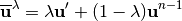
where  are coefficients used to vary the
time-centering of the velocities. The averaging for the hydrostatic
pressure
are coefficients used to vary the
time-centering of the velocities. The averaging for the hydrostatic
pressure  is discussed in
Sec. Hydrostatic Pressure. To maintain an accurate time
discretization of geostrophic balance, it is important that, in the
averaging over the three time levels, the velocity and pressure are
centered at the same time, i.e. if they are centered at time
, then the coefficients for the variables at times
is discussed in
Sec. Hydrostatic Pressure. To maintain an accurate time
discretization of geostrophic balance, it is important that, in the
averaging over the three time levels, the velocity and pressure are
centered at the same time, i.e. if they are centered at time
, then the coefficients for the variables at times
 and
and  must be equal.
2) Next the vertical average of is subtracted. The
result is the baroclinic velocity:
(68)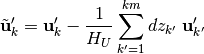
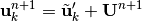
3) Finally, the barotropic system is solved for the barotropic velocity
at the new time  (see
Sec. Barotropic Equations), and this is added to the normalized
auxiliary velocities to obtain the full velocities at the new time:
(see
Sec. Barotropic Equations), and this is added to the normalized
auxiliary velocities to obtain the full velocities at the new time:
(69)
The barotropic velocity is defined by
(70)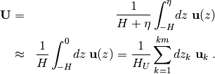
where is the displacement of the free surface relative to
. As discussed in Secs. Barotropic Equations and
Variable-Thickness Surface Layer, in the current version of the POP model we assume
 and approximate the barotropic velocity as the
vertical integral from
and approximate the barotropic velocity as the
vertical integral from  to in (70).
5.4. Baroclinic Momentum Equations
The time discretization of the baroclinic momentum equations for leapfrog steps is given by (65). For forward and backward steps, the time discretization is
Forward steps:
(71)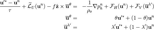
Backward steps:
(72)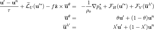
where , and  is the predicted
hydrostatic pressure from the forward step. is the
unnormalized momentum, as in (65) and (68), and
is the predicted
hydrostatic pressure from the forward step. is the
unnormalized momentum, as in (65) and (68), and
 is the same quantity predicted by the forward step
only.
is the same quantity predicted by the forward step
only.  is hardwired into the code. This choice was
made (rather than choosing
is hardwired into the code. This choice was
made (rather than choosing  where both Coriolis and
pressure gradient would be centered and time ) because the
forward step is unstable if the Coriolis terms is treated explicitly.
where both Coriolis and
pressure gradient would be centered and time ) because the
forward step is unstable if the Coriolis terms is treated explicitly.
5.4.1. Pressure Averaging
The method of Brown and Campana (1978) is used for the semi-implicit treatment of the hydrostatic pressure gradient on leapfrog timesteps, where the averaging of the pressure over the three time levels in (65) is given by
(73)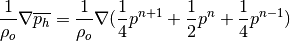
This choice of coefficients allows for a factor of two increase in the CFL limit associated with internal gravity waves, and hence a factor of two increase in timestep if internal gravity waves are the controlling factor (see Maltrud et al. (1998), (1998), for a simple proof of this property).
The new pressure at time is obtained by updating the
tracer transport equations for the temperature and
salinity before the baroclinic momentum equations are solved.
Then the density and hydrostatic pressure at the new time can be
diagnosed from the equation of state and the hydrostatic equation. The
convective adjustment is done afterwards and this modifies the new
and and hence the new pressure. So, in this
case the new pressure before convective adjustment is used in
(73). With implicit vertical mixing the vertical loops over
tracer and momentum are separated, and the implicit vertical diffusion
of tracers is done after the tracer loop and before the momentum loop,
so in that case the exact pressure at the new time is used in
(73). Equation (73) applies to leapfrog
timesteps. On forward steps the time pressure is used, and on
backward steps the predicted pressure from the first pass is used (see
(71), (72)).
5.4.2. Semi-Implicit Treatment of Coriolis and Vertical Friction Terms
A semi-implicit treatment of the Coriolis terms can allow a somewhat longer timestep due to filtering of inertial waves and barotropic Rossby waves, but the main motivation in POP is to damp the Rossby-wave computational mode which appears in the implicit free-surface formulation of the barotropic equations, as shown in Sec. Barotropic Equations and Dukowicz and Smith (1994). Since the barotropic equations are the exact vertical average of the momentum equations, the Coriolis terms in the baroclinic equations must also be treated semi-implicitly. While it is possible to run POP with explicit treatment of the Coriolis terms, we strongly recommend against this because of the above-mentioned computational mode. The following discussion assumes the Coriolis terms are treated semi-implicitly.
The simultaneous semi-implicit treatment of both Coriolis and vertical mixing terms leads to a coupled system where both components of velocity must be solved for simultaneously. To avoid this, we employ an operator splitting which maintains the second-order accuracy of the time discretization. To illustrate this splitting, we write the momentum equations in the matrix form
(74)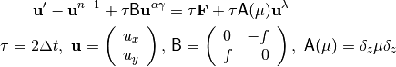
where  is the velocity vector organized in block form and
 is a 2
 2 matrix in the space of the two
velocity components.
2 matrix in the space of the two
velocity components.  represents all other terms in the
momentum equation that are treated explicitly (advection, metric,
pressure gradient and horizontal diffusion terms). The time-averaging of
the velocities
represents all other terms in the
momentum equation that are treated explicitly (advection, metric,
pressure gradient and horizontal diffusion terms). The time-averaging of
the velocities  and
and
 are given by (66) and
(67). Equation (74) can be rewritten as
are given by (66) and
(67). Equation (74) can be rewritten as
![[{\bf I} - \lambda\tau{\sf A}(\mu) + \alpha\tau{\sf B}]
\Delta{\bf u} = \tau \mathbf{F'} \nonumber](../_images/math/d9fe7c8541c4c02d90000c42285a2f6810a2bdac.png)
![\mathbf{F'} \equiv
\{ {\bf F} - {\sf B}[\gamma{\bf u}^n + (1-\gamma){\bf u}^{n-1}]
+{\sf A}(\mu){\bf u}^{n-1}\} \nonumber](../_images/math/426e598a521a11ac5c720437158560784e683d9d.png)
(75)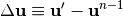
where  is the identity matrix. The operator splitting is
given by
is the identity matrix. The operator splitting is
given by
(76)¶![\begin{aligned}
[{\bf I} - \lambda\tau{\sf A}(\mu) + \alpha\tau{\sf B}]
= [{\bf I} + \alpha\tau{\sf B}]
[{\bf I} - \lambda\tau{\sf A}(\mu) ]
+ {\cal O}(\tau^2)
\end{aligned}](../_images/math/34e47b66c5de2734230b6d3e05d5123f31449dae.png)
and thus second-order accuracy in time is maintained by dropping the
 terms and solving the simpler system
(77)¶![\begin{aligned}
[{\bf I} - \lambda\tau{\sf A}(\mu) ]\Delta{\bf u}
= ({\bf I} + \alpha\tau{\sf B})^{-1}\tau{\bf F}'
\end{aligned}](../_images/math/b303b92120cbc95879d3fea9c66484bf7211c585.png)
The r.h.s. of (77) can be evaluated analytically using
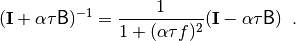
Note again that the surface forcing is contained only on the r.h.s. of
(77). Furthermore, the quadratic bottom drag term
(50) is evaluated at the lagged time and also
appears only on the r.h.s. By lagging the bottom drag term, the
tridiagonal systems for and are linearized and
decoupled, which greatly facilitates their solution. Again,
is the explicit vertical mixing case. For implicit
vertical mixing,  is required, and the code is
typically run with
is required, and the code is
typically run with  . In the barotropic equations
(Sec. Barotropic Equations) we choose
. In the barotropic equations
(Sec. Barotropic Equations) we choose  ,
which is hardwired in the code, and it is clear from (66)
that the Coriolis terms are centered at time .
,
which is hardwired in the code, and it is clear from (66)
that the Coriolis terms are centered at time .
On forward and backward steps the splitting is given by
Forward step:
(78)¶![\begin{aligned}
{\bf u}'^* - {\bf u}^{n} + \tau {\sf B}\overline{{\bf u}}^{\theta}
& = \tau {\bf F} + \tau {\sf A}(\mu)\overline{{\bf u}}^{\lambda'}
\nonumber \\
& \mathrm{or} \nonumber \\
[{\bf I} - \lambda'\tau{\sf A}(\mu) + \theta\tau{\sf B}]
\Delta{\bf u} & = \tau [{\bf F}^n - {\sf B}{\bf u}^n
+{\sf A}(\mu){\bf u}^{n}]
\nonumber \\
\Delta{\bf u} & \equiv {\bf u}'^* - {\bf u}^{n}
\end{aligned}](../_images/math/5b4a08a05b18d4916e79dc59ba083eede05bb0ef.png)
Backward step:
(79)¶![\begin{aligned}
{\bf u}' - {\bf u}^{n} + \tau {\sf B}\overline{{\bf u}}^{\theta}
& = \tau {\bf F} + \tau {\sf A}(\mu)\overline{{\bf u}}^{\lambda'}
\nonumber \\
& \mathrm{or} \nonumber \\
[{\bf I} - \lambda'\tau{\sf A}(\mu) + \theta\tau{\sf B}]
\Delta{\bf u} & = \tau [ {\bf F}^* - {\sf B}{\bf u}^n
+{\sf A}(\mu){\bf u}^{n}] \nonumber \\
\Delta{\bf u} & \equiv {\bf u}' - {\bf u}^{n}
\end{aligned}](../_images/math/c2e1090c50d39447613dab6400c4ee442b214126.png)
where ,  represents the
advection and hydrostatic pressure gradient terms evaluated at time
, and
represents the
advection and hydrostatic pressure gradient terms evaluated at time
, and  represents the same terms evaluated
using the predicted variables from the forward step. In
(78) and (79)
represents the same terms evaluated
using the predicted variables from the forward step. In
(78) and (79)
 is defined as in
(71) and (72), respectively.
Now employing the operator splitting
is defined as in
(71) and (72), respectively.
Now employing the operator splitting
(80)¶![\begin{aligned}
[{\bf I} - \lambda'\tau{\sf A}(\mu) + \theta\tau{\sf B}]
= [{\bf I} + \theta\tau{\sf B}]
[{\bf I} - \lambda'\tau{\sf A}(\mu) ]
+ {\cal O}(\tau^2)
\end{aligned}](../_images/math/302db1ae6794d8967dbc18ba0bdeb32c775d834a.png)
the tridiagonal systems analogous to (77) are:
Forward step:
![[{\bf I} - \lambda'\tau{\sf A}(\mu) ]\Delta{\bf u}
= ({\bf I} + \theta\tau{\sf B})^{-1}\tau[{\bf F}^n
- {\sf B}{\bf u}^n +{\sf A}(\mu){\bf u}^{n}]
\nonumber](../_images/math/2feceaa0addf29d925968d7843df60e69f11ac56.png)
(81)
Backward step:
![[{\bf I} - \lambda'\tau{\sf A}(\mu) ]\Delta{\bf u}
= ({\bf I} + \theta\tau{\sf B})^{-1}\tau[{\bf F}^*
- {\sf B}{\bf u}^n +{\sf A}(\mu){\bf u}^{n}]
\nonumber](../_images/math/cb38e2333e89a661df418ae0c74a4a6454c02a9f.png)
(82)
Again,  is hardwired into the code.
5.5. Barotropic Equations
POP uses the implicit free-surface formulation of the barotropic equations developed by Dukowicz and Smith (1994), and this formulation is presented here. Other possible options are the rigid-lid streamfunction approach (Bryan 1969), the rigid-lid surface pressure approach (Smith, Dukowicz, and Malone 1992; Dukowicz, Smith, and Malone 1993), and the explicit free-surface method (Killworth et al. 1991), which involves subcycling the barotropic mode with a smaller timestep than that used in the baroclinic equations.
The prognostic equation for the barotropic velocity, defined by (70), is obtained by vertically integrating the momentum and continuity equations. The barotropic momentum equation in block form, analogous to (74), is given by:
(83)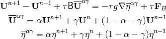
where  is the surface height, and
 is the vertical integral of all terms besides the
time-tendency, Coriolis, and surface pressure gradient terms in the
momentum equation.
is the vertical integral of all terms besides the
time-tendency, Coriolis, and surface pressure gradient terms in the
momentum equation.
5.5.1. Linear Free Surface Model
A prognostic equation for the free surface height is
obtained by vertically integrating the continuity equation
(84)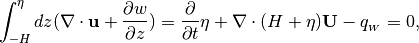
where we have used the surface boundary condition on the vertical velocity:
(85)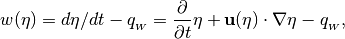
and  is the vertically averaged horizontal velocity:
(86)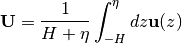
where  and
and  are the vertical and
horizontal velocities at the surface, and
are the vertical and
horizontal velocities at the surface, and  is freshwater
flux. This result is derived using Leibnitz’s Theorem to interchange the
order of integration and differentiation. A difficulty with this form of
the barotropic continuity equation is that, in the implicit time
discretization of the barotropic equations, the term proportional to
inside the divergence in (84) leads to
a nonlinear elliptic system, and standard solution methods such as
conjugate gradient algorithms cannot be directly applied to it. To avoid
this, POP uses a linearized form of the barotropic continuity equation
which is derived as follows. Integrating the continuity equation over
depth as before, but modifying the boundary condition (85)
by dropping the term involving
is freshwater
flux. This result is derived using Leibnitz’s Theorem to interchange the
order of integration and differentiation. A difficulty with this form of
the barotropic continuity equation is that, in the implicit time
discretization of the barotropic equations, the term proportional to
inside the divergence in (84) leads to
a nonlinear elliptic system, and standard solution methods such as
conjugate gradient algorithms cannot be directly applied to it. To avoid
this, POP uses a linearized form of the barotropic continuity equation
which is derived as follows. Integrating the continuity equation over
depth as before, but modifying the boundary condition (85)
by dropping the term involving  (which can be shown to
be of order
(which can be shown to
be of order  relative to the time tendency term), we
find:
relative to the time tendency term), we
find:
(87)
(88)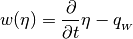
(89)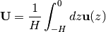
To obtain the linearized barotropic continuity equation we drop the
term  in
(87), which corresponds to neglecting the
horizontal mass flux between and
in
(87), which corresponds to neglecting the
horizontal mass flux between and  :
:
(90)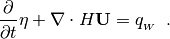
This derivation makes it clear that in the advection operators the
horizontal mass flux between and must be
neglected in order to be consistent with (90). So
there are four ingredients to the linear free surface model: 1) the
barotropic continuity equation is given by (90)
instead of (84); 2) the barotropic velocity is
given by (89) instead of (86); 3)
the vertical velocity at the surface, which is used to integrate the
continuity equation from the top down, is given by (88)
instead of (85); and 4) the horizontal mass fluxes between
and should be neglected in the advection
operators and when integrating the continuity equation to find the
vertical velocities. In the discrete equations this means that the
horizontal mass fluxes in the surface cells are proportional to the full
cell height  , rather than
  (see Sec.
Variable-Thickness Surface Layer). This linear approximation is valid provided the
surface displacement is small compared to the depth of the full ocean:
(see Sec.
Variable-Thickness Surface Layer). This linear approximation is valid provided the
surface displacement is small compared to the depth of the full ocean:
 , and in the discrete equations the surface
displacement must also be small compared to the depth of the surface
layer:
, and in the discrete equations the surface
displacement must also be small compared to the depth of the surface
layer:  .
.
With a non-zero freshwater flux the mean volume of the
ocean is not constant, even though the velocity field is divergence
free. Integrating (90) over horizontal area, we
find
(91)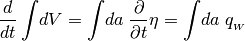
where  is the horizontal area element. So the total
volume of the ocean will change unless the surface-integrated freshwater
flux vanishes.
is the horizontal area element. So the total
volume of the ocean will change unless the surface-integrated freshwater
flux vanishes.
5.5.2. Time Discretization of the Barotropic Equations
In the implicit free-surface formulation the continuity equation (90) is discretized in time using a forward step as follows:
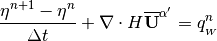
(92)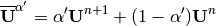
where  is a coefficient used to vary the time centering
of the velocity in the continuity equation. The barotropic equations
support three types of linear waves: two gravity waves (one in each
horizontal direction) and one Rossby wave. In a pure leapfrog
discretization, there would be three computational modes, one associated
with each of these waves. By choosing the forward discretization
(92), one computational mode is eliminated, leaving
one gravity-like and one Rossby-like computational mode. The Rossby
computational mode is damped by the discretization scheme if the
Coriolis terms are treated implicitly, and the gravity-wave
computational mode is strongly damped if is close to 1.
In Dukowicz and Smith (1994) it was shown that the optimal set of
time-centering coefficients which maximally damps the computational
modes, minimally damps the physical modes, and minimally distorts the
phase speed of the physical modes is given by the parameter set:
is a coefficient used to vary the time centering
of the velocity in the continuity equation. The barotropic equations
support three types of linear waves: two gravity waves (one in each
horizontal direction) and one Rossby wave. In a pure leapfrog
discretization, there would be three computational modes, one associated
with each of these waves. By choosing the forward discretization
(92), one computational mode is eliminated, leaving
one gravity-like and one Rossby-like computational mode. The Rossby
computational mode is damped by the discretization scheme if the
Coriolis terms are treated implicitly, and the gravity-wave
computational mode is strongly damped if is close to 1.
In Dukowicz and Smith (1994) it was shown that the optimal set of
time-centering coefficients which maximally damps the computational
modes, minimally damps the physical modes, and minimally distorts the
phase speed of the physical modes is given by the parameter set:
(93)
Thus in (83)
and similarly for  . These
choices are hardwired into the code. The physical gravity waves are
damped at small space and time scales in this implicit scheme, but the
physical Rossby waves are essentially unaffected.
. These
choices are hardwired into the code. The physical gravity waves are
damped at small space and time scales in this implicit scheme, but the
physical Rossby waves are essentially unaffected.
By inserting the barotropic momentum equation (83) into the
continuity equation (92) we obtain an elliptic
equation for the surface height at the new time .
However, due to the presence of the Coriolis terms, the resulting
elliptic operator is not symmetric, making it much more difficult to
invert, because standard solvers such as conjugate gradient methods
require symmetric positive-definite linear operators. This problem can
be overcome by using an operator splitting technique that maintains the
second-order accuracy of the time discretization scheme (Smith,
Dukowicz, and Malone 1992; Dukowicz, Smith, and Malone 1993). Defining
an auxiliary velocity
(94)
equation (83) can be written:
(95)¶![\begin{aligned}
({\bf I} + \alpha\tau{\sf B})(\hat{\bf U} - {\bf U}^{n-1})
& =\tau\{{\bf F}_B -
{\sf B}[\gamma{\bf U}^n + (1-\gamma){\bf U}^{n-1}] \nonumber \\
& - g\nabla[\gamma\eta^n + (1-\gamma)\eta^{n-1}]\}
+{\cal O}(f\tau^3)
\end{aligned}](../_images/math/9eee8537fe6123bf1e44c96eee64d3e8152da7c6.png)
Dropping the  terms (which are the same order
as the time truncation error in this second-order scheme), and using the
continuity equation (92) with
terms (which are the same order
as the time truncation error in this second-order scheme), and using the
continuity equation (92) with  , we
arrive at the elliptic system
, we
arrive at the elliptic system
(96)¶![{\big [} \nabla\cdot H\nabla - \frac{1}{g\alpha\tau\Delta t}
\big] \eta^{n+1} =
\nabla\cdot H\big[\frac{\hat{\bf U}}{g\alpha\tau}
+\nabla\eta^{n-1} \big] - \frac{\eta^{n}}{g\alpha\tau\Delta t}
-\frac{q^n_{_W}}{g\alpha\tau}](../_images/math/ee915df9c474fd8545db67f6ccd39be993c2c5d2.png)
The procedure is to first solve (95) for  ,
then solve (96) for (POP actually solves
for the surface pressure
,
then solve (96) for (POP actually solves
for the surface pressure  ), and finally use
(94) to obtain . This system is solved in
POP on leapfrog timesteps with
), and finally use
(94) to obtain . This system is solved in
POP on leapfrog timesteps with  using a diagonally
preconditioned conjugate gradient algorithm described in Sec. Conjugate Gradient Algorithm.
Note that the terms dropped in (95) are only
using a diagonally
preconditioned conjugate gradient algorithm described in Sec. Conjugate Gradient Algorithm.
Note that the terms dropped in (95) are only
 if the timestep is small compared to the
inertial period
if the timestep is small compared to the
inertial period  . We therefore recommend that the model
timestep be no greater than about two hours. The scheme is stable for
longer timesteps, but the barotropic mode will start to become
inaccurate as the timestep is increased above two hours. The divergence
on the r.h.s. in (96) is discretized with the correct
B-grid discretization, i.e., the quantity in brackets is transversely
averaged as in (33). The Laplacian-like operator on the l.h.s. in
(96) is a nine-point stencil with the correct B-grid
discretization:
. We therefore recommend that the model
timestep be no greater than about two hours. The scheme is stable for
longer timesteps, but the barotropic mode will start to become
inaccurate as the timestep is increased above two hours. The divergence
on the r.h.s. in (96) is discretized with the correct
B-grid discretization, i.e., the quantity in brackets is transversely
averaged as in (33). The Laplacian-like operator on the l.h.s. in
(96) is a nine-point stencil with the correct B-grid
discretization:
(97)¶![\nabla\cdot H\nabla\eta =
\frac{1}{\Delta_y} \delta_x
\overline{\big[\Delta_y H_U\delta_x \overline{\eta}^y \big]}^y
+ \frac{1}{\Delta_x} \delta_y
\overline{\big[\Delta_x H_U\delta_y \overline{\eta}^x \big]}^x.](../_images/math/ec05c0f89c10f2d7c3a4473a593e7dfe0f4758d1.png)
Unlike the friction and diffusion operators, this operator cannot be approximated as a five-point stencil, because doing so would violate the energetic balance between pressure work and change in potential energy (see Sec. Energetic Consistency). Since the nine-point B-grid operator in (97) has a checkerboard null space (see Sec. Nullspace Removal), the solution of (96) is prone to have local patches of checkerboard noise. Strictly speaking, the operator on the l.h.s. of (96) has no checkerboard null space due to the presence of the extra diagonal term (second term in brackets). However, if the solution in some region is in a near steady state, this diagonal term is cancelled by the next to last term on the r.h.s., and checkerboard noise may appear. This is particularly true in isolated bays where the solution is only weakly coupled to the interior. On the other hand, the checkerboard noise has little effect on the dynamics because only the gradient of surface height enters the barotropic momentum equation, and the B-grid gradient operator (33) does not see a checkerboard field. The only way a checkerboard surface height field can affect the dynamics is through the vertical velocity at the surface (39), which depends on the change in surface height, and is used as the surface boundary condition to integrate the continuity equation to find the advection velocities. However, experience has so far shown that this does not lead to serious problems with the model simulations.
It should be noted that the solution for surface height will only
satisfy the continuity equation (92) to the extent
that the solution of (96) has converged in the iterative
solution of the elliptic solver. As discussed in
Sec. Tracer Advection, this can lead to a small non-divergent mass
flux in the bottom-most ocean cell when the 3-D continuity equation is
integrated from the top down with given by (88)
at the surface, as discussed in Sec. Tracer Advection. In
practice, we suggest that the convergence criterion for the iterative
solver be chosen so that the global mean balance between pressure work
and change in potential energy is accurate to within about three
significant digits (see Sec. Energetic Consistency on energetic
consistency).
The time discretization for forward and backwards steps, corresponding to (83) and (92) are given by:
Forward step:

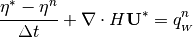
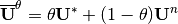
(98)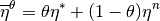
Backward step:

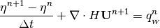
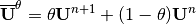
(99)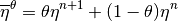
where we have assumed  as in
(92) and (93).
as in
(92) and (93).  and
and
 are the predicted barotropic velocity and surface height
from the forward step.
are the predicted barotropic velocity and surface height
from the forward step.  contains all terms other than
the Coriolis, surface pressure gradient and time-tendency terms in the
barotropic momentum equation, all evaluated at time , and
contains all terms other than
the Coriolis, surface pressure gradient and time-tendency terms in the
barotropic momentum equation, all evaluated at time , and
 contains the same terms but evaluated using the
prognostic variables predicted by the forward step. The operator
splittings for the forward and backward steps, analogous to
(94) and (95) are:
contains the same terms but evaluated using the
prognostic variables predicted by the forward step. The operator
splittings for the forward and backward steps, analogous to
(94) and (95) are:
Forward step:
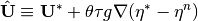
(100)
Backward step:

(101)¶![({\bf I} + \theta\tau{\sf B})(\hat{\bf U} - {\bf U}^{n})
=\tau\{{\bf F}^*_B - {\sf B}{\bf u}^n
- g[\theta\nabla\eta^* +(1-\theta)\nabla\eta^n]\}
+{\cal O}(f\tau^3)](../_images/math/c6b1382948b85c69f711c154caec88cb8391ea9f.png)
Finally, the elliptic equations for the forward and backward steps analogous to (96) are given by:
Forward step:
(102)¶![{\big [} \nabla\cdot H\nabla - \frac{1}{g\theta\tau\Delta t}
\big] \eta^* =
\nabla\cdot H\big[\frac{\hat{\bf U}}{g\theta\tau}
+\nabla\eta^{n} \big] - \frac{\eta^{n}}{g\theta\tau\Delta t}
-\frac{q^n_{_W}}{g\theta\tau}](../_images/math/283970005d879f5d101a56e714b48f25b2218fa4.png)
Backward step:
(103)¶![{\big [} \nabla\cdot H\nabla - \frac{1}{g\theta\tau\Delta t}
\big] \eta^{n+1} =
\nabla\cdot H\big[\frac{\hat{\bf U}}{g\theta\tau}
+\nabla\eta^* \big] - \frac{\eta^{n}}{g\theta\tau\Delta t}
-\frac{q^n_{_W}}{g\theta\tau}](../_images/math/e88666b2c838d68b5dda078eac0f4352b2e820d5.png)
5.5.3. Conjugate Gradient Algorithm
The most efficient method we have found for solving the elliptic system
of barotropic equations (96) is to use a standard
Preconditioned Conjugate Gradient solver. The algorithm consists of the
following steps to solve the system  given by
(96) multiplied by the T-cell area.
given by
(96) multiplied by the T-cell area.  is the
symmetric positive-definite Laplacian type operator on the l.h.s. in
(96) (it is important to note that if (96) is
not multiplied by the T-cell area then the operator is not symmetric),
is the
symmetric positive-definite Laplacian type operator on the l.h.s. in
(96) (it is important to note that if (96) is
not multiplied by the T-cell area then the operator is not symmetric),
 is the r.h.s., and is the solution. Lower-case Greek
and Roman letters are used, respectively for scalars and 2-D arrays, and
is the r.h.s., and is the solution. Lower-case Greek
and Roman letters are used, respectively for scalars and 2-D arrays, and
 denotes a dot product:
 .
.
PCG Algorithm:
Initial guess:
Compute initial residual
Set
,
For
do
Exit if converged:
End do


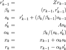
Here  is a preconditioning matrix. This is usually taken to be
a diagonal preconditioner
is a preconditioning matrix. This is usually taken to be
a diagonal preconditioner  , where
  is the
diagonal matrix composed of the central coefficient in the nine-point
stencil corresponding to the operator in (96). The code is
set up to use a more sophisticated preconditioner consisting of a
nine-point operator which is a local approximate inverse of the true
operator (Smith, Dukowicz, and Malone 1992). This preconditioner is
expensive to compute but is time independent and can be computed offline
and read in by the code. To improve the initial guess,
is the
diagonal matrix composed of the central coefficient in the nine-point
stencil corresponding to the operator in (96). The code is
set up to use a more sophisticated preconditioner consisting of a
nine-point operator which is a local approximate inverse of the true
operator (Smith, Dukowicz, and Malone 1992). This preconditioner is
expensive to compute but is time independent and can be computed offline
and read in by the code. To improve the initial guess,  is
linearly extrapolated in time from the solutions at the two previous
timesteps. In the convergence criterion
is
linearly extrapolated in time from the solutions at the two previous
timesteps. In the convergence criterion
 ,
,
 is the rms T-cell area. This normalization is
somewhat arbitrary, but is chosen so that
is the rms T-cell area. This normalization is
somewhat arbitrary, but is chosen so that  has the same
dimensions as the operator (96) before it is multiplied by
the T-cell area averaged over surface ocean points. As discussed in
Sec. Time Discretization of the Barotropic Equations, we suggest that be chosen
such that the global mean balance between pressure work and change in
potential energy is accurate to within about three significant digits.
Typically this is achieved for values of between
10
has the same
dimensions as the operator (96) before it is multiplied by
the T-cell area averaged over surface ocean points. As discussed in
Sec. Time Discretization of the Barotropic Equations, we suggest that be chosen
such that the global mean balance between pressure work and change in
potential energy is accurate to within about three significant digits.
Typically this is achieved for values of between
10 and 10
 .
.
The conjugate gradient solver outlined above has poor scalability on many distributed memory computer systems. The fundamental limit to scalability is the need for three dot products, each requiring a global summation operation and adding an inherent sychronization. A variant of the standard conjugate gradient solution method, known as the Chronopoulos-Gear algorithm (D’Azevedo, Eijkhout, and Romine 1993), combines the separate global sums into a single vector global sum, which reduces the latency to one third. This option is now the default in POP, though the previous PCG algorithm is still supported.
6. Grids
6.1. Global Orthogonal Grids
As discussed in Sec. Spatial Discretization, the POP model is designed to
handle any orthogonal curvilinear coordinate system for the horizontal
grid. The only information the code needs locally at each grid point is
the longitude and latitude of velocity points and the distances to
neighboring points along the two coordinate directions. This information
is computed offline and read in from a file. However, there are
restrictions on the global connectivity of the grid. In the current
model release, it is assumed that the computational grid can be mapped
onto a 2-D domain. When such global grids are mapped onto the sphere
they necessarily involve two singularities, analogous to the north and
south poles on a standard polar grid. In these ``dipole” grids,
originally developed independently by two groups (Madec and Imbard 1996;
Smith, Kortas, and Meltz 1995), the two singularities can be placed
inside land masses (e.g., North America, Greenland or Asia) to construct
global grids. POP also has the ability to use what we call “tripole”
grids, which were originally developed by Murray (1996). In these grids,
there are two “poles” in the northern hemisphere (usually placed in
North America and Asia). These grids can also be mapped onto a cylinder
but special boundary communications are required in order to “sew up”
the line between the two northern poles. In both dipole and tripole
grids, the meshes are constructed so that there is a smooth transition
moving north from the Equator, from the southern hemisphere polar grid
(usually Mercator grid) to the northern “distorted” grid. Various
factors enter into the design of a given grid, and different choices
(pole locations, dipole vs. tripole) may be preferred for different
problems. In global grids the Equator is typically chosen as a grid line
so that the numerical dispersion relation for the B-grid linear Kelvin
waves is accurate. At resolutions coarser than about
 , the meridional spacing near the Equator is
enhanced (to about ) in order to more
accurately resolve equatorial waves and currents. Note: Software for
generation of global dipole and tripole grids is not released with the
code, but will eventually be made public.
, the meridional spacing near the Equator is
enhanced (to about ) in order to more
accurately resolve equatorial waves and currents. Note: Software for
generation of global dipole and tripole grids is not released with the
code, but will eventually be made public.
6.1.1. Dipole Grids
The simplest orthogonal grid with two arbitrarily located poles can be constructed analytically in one of three ways:
- Electrostatic dipole charge distribution on a sphere: solve Poisson’s Equation on the sphere with two electric charges of opposite sign at the chosen pole points; the electric field lines and the lines of constant electrostatic potential form an orthogonal coordinate system;
- Conformal map method (Murray 1996): project a spherical polar grid onto a tangent plane at its equator from the point on the sphere opposite the tangent point, then reproject back onto a larger sphere tangent to the plane at the same point; the new pole points on the larger sphere will be shifted toward its equator and the tangent point;
- Geometric method (Smith, Kortas, and Meltz 1995): choose two axes, one which intersects the surface of the sphere at the two pole points and one located at the intersection of the two planes tangent to the pole points, then the two families of planes that contain these axes intersect the surface of the sphere in two sets of circles which form the coordinates of an orthogonal coordinate system.
All these methods produce equivalent orthogonal grids. The only problem with these simple analytic grids is that if one pole is located in Antarctica and the other is displaced away from the true North Pole, then the Equator will not be a grid line. To get around this problem, grids can be constructed by an iterative procedure (Madec and Imbard 1996; Smith, Kortas, and Meltz 1995), starting at the equator of a southern hemisphere polar grid, where the northern pole point is gradually shifted away from the true North Pole as successive latitude-like circles are constructed. In this manner it is possible to construct a semi-analytic dipole grid which smoothly matches onto the southern polar grid, and in which local changes in grid spacing are everywhere small and smooth. Composite grids that have sudden changes in grid spacing normal to matching boundaries suffer a loss of formal second-order accuracy of the spatial discretization scheme (Smith, Kortas, and Meltz 1995).
An example of a semi-analytic dipole grid is shown in Figure5.1 . In this grid the northern pole is in North America and the southern hemisphere is a Mercator grid with a pole at the true South Pole. Note that the meridional grid spacing near the Equator has been enhanced as discussed above. The grid spacing in the northern hemisphere is chosen so as to minimize the global mean aspect ratio, attempting to make each cell as nearly “square” as possible (as in a true Mercator grid). In both hemispheres the grid terminates in a circle enclosing the pole, and anything within this circle is excluded (e.g., Hudson Bay in Figure5.1.
Figure 5.1 A dipole grid.
6.1.2. Tripole Grids
Analytic grids can also be constructed which involve more than two
singularities using the different methods described above for dipole
grids. Various types of multipole grids are discussed by Murray (1996).
One variation that is particularly useful for ocean models is shown in
Figure 11 of Murray (1996). It has two singularities in the northern
hemisphere and smoothly matches onto a southern hemisphere Mercator
grid. A “tripole” grid of this type is shown in Figure5.2 .
Note that the grid spacing in the Arctic is much more uniform and the
cell aspect ratios are much closer to one than in the dipole grid in
Figure5.1 . This particular grid was constructed for the French
OPA model (Madec, Imbard, and Levy 1998), and was made available,
courtesy of G. Madec, for testing in POP. Like the dipole grid, the
tripole grid is mapped onto a cylinder (a logical 2-D array that is
periodic in the direction). The difference is that in the
dipole grid the northernmost (``upper”) boundary of the grid
corresponds to the circle surrounding the pole (e.g. the open circle
containing Hudson bay in Figure5.1 ), whereas in the tripole grid
the two northern poles both lie on the upper boundary, one is located at
the two upper corners of the logical grid (which correspond to the same
point because it is periodic) and the other at the midpoint of the upper
boundary. When the 2-D cylindrical array is mapped onto the sphere (as
in Figure5.2 ) there is a chopped pole in the southern
hemisphere, but in the northern hemisphere there is a “cut” in the grid
along the line between the poles, and flow across this line from one
side of the Arctic to the other requires non-local communication along
the upper boundary of the logical grid: it must be folded back along
itself at its mid point in order to make neighboring cells in the
physical grid be adjacent in the logical grid. The indexing for this
nonlocal communication is different for quantities located at different
places (i.e. U-points or T-points) on the grid. POP does assume that in
the logical grid the upper boundary lies on the northern edge of the
last row of T-cells, so that U-points lie exactly on the upper grid
boundary, along the line between the two poles. Furthermore, it assumes
that the middle pole point lies at a U-point exactly halfway across the
top of the grid.
Figure 5.2: A tripole grid.
6.2. Vertical Grid Variants
The current vertical grid in POP is a fixed Eulerian grid with depth as the vertical coordinate. However, two options are available to mitigate some problems encountered with such a grid. A variable-thickness surface layer can be used to more accurately treat changes in sea surface height and fluxes of tracers at the surface. Partial bottom cells can be used to more accurately represent bottom topography.
6.2.1. Variable-Thickness Surface Layer
The tracer transport equations have the form
(104)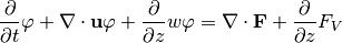
where  and
and
 are, respectively,
the horizontal and vertical diffusion operators. Integrating this
equation over the model surface level (from
are, respectively,
the horizontal and vertical diffusion operators. Integrating this
equation over the model surface level (from  to
, where
to
, where  is the depth of the upper level)
we find:
is the depth of the upper level)
we find:
(105)
In deriving (105) the same approximations used in the
linear free surface model (Sec. Linear Free Surface Model) were
employed: the boundary condition (88) was applied, and the
advective and diffusive horizontal fluxes between and
were set to zero. Note that there is no advection of
tracers through the surface with the vertical velocity .
Some care must be taken to specify the tracer fluxes through the air-sea interface. The total tracer flux seen by the ocean model at the surface is given by
(106)
where  is the tracer concentration at the sea
surface and
is the tracer concentration at the sea
surface and  represents the advection of
tracers in the ocean relative to the sea surface due to the freshwater
flux. The atmosphere (or sea ice model) sees a flux of tracers into the
ocean given by
represents the advection of
tracers in the ocean relative to the sea surface due to the freshwater
flux. The atmosphere (or sea ice model) sees a flux of tracers into the
ocean given by
(107)
where  is the tracer concentration in the
freshwater being added or removed from the ocean, (for simplicity we
assume here that locally there will be only one source of freshwater,
and omit the sum over different types freshwater sources – see (36)),
and is any additional flux of tracers (e.g., for
temperature in the open ocean it corresponds to the sum of sensible,
latent, shortwave and longwave heat fluxes). In reality there is a very
thin boundary layer where the tracer concentration varies continuously
and
is the tracer concentration in the
freshwater being added or removed from the ocean, (for simplicity we
assume here that locally there will be only one source of freshwater,
and omit the sum over different types freshwater sources – see (36)),
and is any additional flux of tracers (e.g., for
temperature in the open ocean it corresponds to the sum of sensible,
latent, shortwave and longwave heat fluxes). In reality there is a very
thin boundary layer where the tracer concentration varies continuously
and  at the interface. The models do
not resolve this boundary layer and so in general
at the interface. The models do
not resolve this boundary layer and so in general
 . However, the total flux must be
conserved across the boundary layer, so that
. However, the total flux must be
conserved across the boundary layer, so that  , and this
can be used to eliminate in terms of
. Substituting (107) for (106) in
(105), we obtain
, and this
can be used to eliminate in terms of
. Substituting (107) for (106) in
(105), we obtain
(108)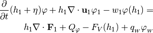
where now the flux  is applied as the surface boundary
condition on . The integrals over the surface layer
have been evaluated by assuming the model variables are constant within
the surface layer.
is applied as the surface boundary
condition on . The integrals over the surface layer
have been evaluated by assuming the model variables are constant within
the surface layer.  is the velocity at the bottom of the
surface layer and
is the velocity at the bottom of the
surface layer and  represents tracer advection
through the bottom of the surface layer. Dividing
(108) by
represents tracer advection
through the bottom of the surface layer. Dividing
(108) by  , we arrive at the tracer
transport equation (34).
, we arrive at the tracer
transport equation (34).
It remains to specify the freshwater tracer concentrations
. In the case of salinity the default choice in the
code is 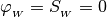 , that is, the freshwater flux
 is assumed to have zero
salinity (where , , , and
are the freshwater fluxes associated with precipitation,
evaporation, river runoff, freezing and melting of sea ice). In the case
of potential temperature, the default is to assume the freshwater has
the same temperature as the model surface layer, so that
is assumed to have zero
salinity (where , , , and
are the freshwater fluxes associated with precipitation,
evaporation, river runoff, freezing and melting of sea ice). In the case
of potential temperature, the default is to assume the freshwater has
the same temperature as the model surface layer, so that
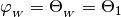 . However, in general the
tracer concentration in the freshwater may vary depending on its source
(precipitation, evaporation, etc.), and the default assumption that
these are all given by a single value as in
(107) may be inadequate. When coupling to atmospheric or
sea-ice models a more accurate accounting of the fluxes may be needed to
ensure they are conserved between component models.
. However, in general the
tracer concentration in the freshwater may vary depending on its source
(precipitation, evaporation, etc.), and the default assumption that
these are all given by a single value as in
(107) may be inadequate. When coupling to atmospheric or
sea-ice models a more accurate accounting of the fluxes may be needed to
ensure they are conserved between component models.
Combining (108) with the transport equations in the subsurface levels and integrating over volume, we find
(109)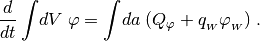
Thus tracers are conserved in the absence of surface fluxes. This is
also true of the time-discretized equations in the model. In particular,
if there are no surface fluxes of salinity,  , and if the
freshwater flux has zero salinity (),
then total salt is conserved.
, and if the
freshwater flux has zero salinity (),
then total salt is conserved.
The time discretization of (108) or (34) is given by (51) for leapfrog steps and by (54) and (55) for forward and backward (Matsuno) timesteps. All of these discrete equations conserve global mean tracers exactly in the sense of (109).
There is also a small error in the time discretization associated with
the fact that we have adopted a three-time-level leapfrog scheme for the
tracer transport equations (51), but a two-time-level
discretization for the barotropic continuity equation
(92). Note that in the limit of a constant tracer
 the continuous transport equation (104), in
the absence of surface forcing, reduces to the continuity equation
the continuous transport equation (104), in
the absence of surface forcing, reduces to the continuity equation
 , and the vertically integrated transport equations
also reduce to the barotropic continuity equation
(90). This does not hold for the discrete
equations because of the inconsistency between the two- and
three-time-level schemes. The consequence of this is that a tracer which
is initially constant in space may evolve to have some small spatial
variations. However, this error is second-order in time and is typically
extremely small. In a test problem involving the Goldsborough-Stommel
circulation (Griffies et al. 2001), which involves only freshwater
forcing at the surface, the temperature field, which is initially
constant, deviates from its initial value by only 1 part in
, and the vertically integrated transport equations
also reduce to the barotropic continuity equation
(90). This does not hold for the discrete
equations because of the inconsistency between the two- and
three-time-level schemes. The consequence of this is that a tracer which
is initially constant in space may evolve to have some small spatial
variations. However, this error is second-order in time and is typically
extremely small. In a test problem involving the Goldsborough-Stommel
circulation (Griffies et al. 2001), which involves only freshwater
forcing at the surface, the temperature field, which is initially
constant, deviates from its initial value by only 1 part in  in a 100-year integration, and furthermore, the error does not
accumulate in time. Therefore, we feel that this error is small enough
that it will not cause problems in long-term climate simulations.
in a 100-year integration, and furthermore, the error does not
accumulate in time. Therefore, we feel that this error is small enough
that it will not cause problems in long-term climate simulations.
Finally, note that the time discretization error when momentum
acceleration is used, see Sec. Tracer Acceleration, may lead to a
computational instability when the variable thickness surface layer
option is used with explicit fresh water fluxes. Because of this
possibility, we advise using the variable thickness surface layer option
with virtual salt fluxes if momentum acceleration, with
 , is being used.
6.2.1.1. Nullspace Removal
The operator for the implicit solution of the barotropic equations for
the surface height in (96) contains the
Laplacian-like term (97). On the B-grid this nine-point
Laplacian-like operator contains two null eigenvectors: a constant field
and a global checkerboard ( or black/white) field (a
checkerboard field has the value of  in black cells and
 in white cells). The Laplacian operator on the B-grid
annihilates both these types of null fields (i.e., they have zero
eigenvalue). On the C-grid, the global checkerboard is not a null
eigenvector; for this reason all the horizontal diffusive operators in
POP have an approximate C-grid discretization, allowing grid-scale
checkerboard noise to be damped by these operators. However, the
presence of a checkerboard component in the surface height field does
not significantly affect the dynamical solution in most cases. The
dominant effect of the surface height is through its contribution to the
surface pressure gradient, and on the B-grid the gradient operator also
does not see the checkerboard field. There is only a small indirect
effect on the vertical velocities in T-columns because they are
determined by vertically integrating the continuity equation with the
surface boundary condition (39), which depends on .
in white cells). The Laplacian operator on the B-grid
annihilates both these types of null fields (i.e., they have zero
eigenvalue). On the C-grid, the global checkerboard is not a null
eigenvector; for this reason all the horizontal diffusive operators in
POP have an approximate C-grid discretization, allowing grid-scale
checkerboard noise to be damped by these operators. However, the
presence of a checkerboard component in the surface height field does
not significantly affect the dynamical solution in most cases. The
dominant effect of the surface height is through its contribution to the
surface pressure gradient, and on the B-grid the gradient operator also
does not see the checkerboard field. There is only a small indirect
effect on the vertical velocities in T-columns because they are
determined by vertically integrating the continuity equation with the
surface boundary condition (39), which depends on .
In the implicit free surface formulation, the extra term on the left in
(96) is a diagonal term associated with the free surface
(the  term in the barotropic continuity
equation). Without this diagonal term, as in the case in the rigid-lid
surface pressure formulation (Smith, Dukowicz, and Malone 1992), the
null eigenvectors are not removed by the operator, and can creep into
the iterative solution. The diagonal term shifts the eigenvalue of both
constant and checkerboard fields away from zero so that they are damped.
Therefore, in most cases it is not necessary to explicitly remove
constant or checkerboard fields from the solution of the implicit
free-surface system. However, experience has shown that the solution
sometimes does develop large but localized regions where checkerboard
noise appears in the surface height. The exact nature of such regional
checkerboarding is not completely understood. It can even occur in the
rigid-lid streamfunction formulation using an approximate five-point
operator for the barotropic operator which has no global checkerboard
nullspace. Note that a five-point approximation is allowed in this case
but not in the surface pressure or free-surface formulations, because
the five-point approximation to the nine-point B-grid operator violates
energetic consistency (Smith, Dukowicz, and Malone 1992). Experience has
also shown that this regional checkerboarding does not affect the
dynamical solution, again because it is almost completely invisible to
the gradient operator. However, with the variable-thickness surface
layer (Sec. Variable-Thickness Surface Layer), such regional checkerboarding can
appear in the solution and then slowly accumulate over time, eventually
leading to large checkerboard components that can affect the solution,
either by contributing a large roundoff error to the pressure gradient,
or by becoming so large that in some cells the surface height descends
below the bottom of the surface layer.
term in the barotropic continuity
equation). Without this diagonal term, as in the case in the rigid-lid
surface pressure formulation (Smith, Dukowicz, and Malone 1992), the
null eigenvectors are not removed by the operator, and can creep into
the iterative solution. The diagonal term shifts the eigenvalue of both
constant and checkerboard fields away from zero so that they are damped.
Therefore, in most cases it is not necessary to explicitly remove
constant or checkerboard fields from the solution of the implicit
free-surface system. However, experience has shown that the solution
sometimes does develop large but localized regions where checkerboard
noise appears in the surface height. The exact nature of such regional
checkerboarding is not completely understood. It can even occur in the
rigid-lid streamfunction formulation using an approximate five-point
operator for the barotropic operator which has no global checkerboard
nullspace. Note that a five-point approximation is allowed in this case
but not in the surface pressure or free-surface formulations, because
the five-point approximation to the nine-point B-grid operator violates
energetic consistency (Smith, Dukowicz, and Malone 1992). Experience has
also shown that this regional checkerboarding does not affect the
dynamical solution, again because it is almost completely invisible to
the gradient operator. However, with the variable-thickness surface
layer (Sec. Variable-Thickness Surface Layer), such regional checkerboarding can
appear in the solution and then slowly accumulate over time, eventually
leading to large checkerboard components that can affect the solution,
either by contributing a large roundoff error to the pressure gradient,
or by becoming so large that in some cells the surface height descends
below the bottom of the surface layer.
When complicated lateral boundaries are included in the computational
mesh, other global null eigenvectors besides the constant and
checkerboard fields can also exist. These occur when the domain contains
quasi-isolated bays that are only connected to the rest of the ocean
through openings of one or two cell faces. These regions can have their
own constant and checkerboard nullspaces. There are two types of
quasi-isolated bays that need to be considered: 1) bays that are
connected to the rest of the ocean at the surface by only one face of a
T-cell, and 2) bays that are connected by two adjacent faces of the same
T-cell, so that the mouth of the bay is across the diagonal of the
T-cell. If either of these types of bay is in the grid, a checkerboard
nullspace component of the solution can accumulate in the bay. In the
first type of bay, a constant nullspace can also accumulate. In these
smaller areas, the problems mentioned above (leading to roundoff error
or complete emptying of surface cells) accumulate more quickly in time.
Normally, bays of the first type do not appear, because it is the usual
practice during construction of a grid to eliminate all points that are
connected to the open ocean by only one cell face (such points have no
influence on the flow except through diffusion across the open face).
But when the variable-thickness surface layer is used, it is necessary
to remove all isolated bays of both types in order for the model to run
stably. Once these bays are eliminated from the grid, it is still
necessary to remove the global constant and checkerboard nullspaces
associated with the full domain, to prevent them from slowly
accumulating over time. The null fields are projected out of the
solution subject to two constraints: 1) the resulting field has no
checkerboard component; and 2) the projection leaves the global mean sea
level unchanged. Denoting the null eigenvectors  and
and  , which are normalized to 1 and
  ,
respectively, the nullspaces can be projected out with the following
operation (here
,
respectively, the nullspaces can be projected out with the following
operation (here  is the surface height field considered
as a one-dimensional vector, and
is the surface height field considered
as a one-dimensional vector, and  is the same field
after the projection):
is the same field
after the projection):
(110)
where  is the one-dimensional vector of cell areas, and
the sums are over all surface cells. It is straightforward to show that
is the one-dimensional vector of cell areas, and
the sums are over all surface cells. It is straightforward to show that
 and
and
 .
The latter constraint ensures the projection does not change the global
mean sea level. This projection is applied once each timestep
immediately after the barotropic equations are solved for .
.
The latter constraint ensures the projection does not change the global
mean sea level. This projection is applied once each timestep
immediately after the barotropic equations are solved for .
6.2.2. Partial Bottom Cells
To better represent the bottom topography, we employ the idea of partial bottom cells introduced by Adcroft, Hill, and Marshall (1997) and later developed for the MOM model by Pacanowski and Gnanadesikan (1998), for which the thickness of bottom cells is allowed to vary in space. When we place tracer or pressure points at the center of partial bottom cells, as shown in Figure5.3 , the finite difference for horizontal derivatives between two adjacent points introduces an error because these points are located at different vertical positions. More specifically, when we compute the horizontal pressure gradient, we have
(111)¶![\begin{aligned}
\left.\frac{\partial p}{\partial x}\,\right\vert_{z=-h(x)}
= \frac{\partial}{\partial x}\left [\, p\,\vert_{z=-h(x)}\right ]
- g\rho\,\vert_{z=-h(x)}\, h(x)\,,
\end{aligned}](../_images/math/12ba439ce4573825204ce565f3e2748650325b1f.png)
where  can be regarded as the position of tracer points.
Without the second term on the right hand side of (111), the pressure
gradient does not vanish even for
can be regarded as the position of tracer points.
Without the second term on the right hand side of (111), the pressure
gradient does not vanish even for  for which we
expect
for which we
expect 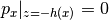 . Even though we include the
correction term,
. Even though we include the
correction term,  vanishes only when
  varies
linearly in depth, because is computed from the hydrostatic
equation
varies
linearly in depth, because is computed from the hydrostatic
equation  by using the trapezoidal rule. Likewise,
when we compute the horizontal diffusion of tracers without taking the
effects of different vertical positions of tracer points into account,
we also introduce spurious diffusion errors. To avoid these errors, the
interpolation between two vertical points has been used in
-coordinate ocean models. More specifically, after finding
by using the trapezoidal rule. Likewise,
when we compute the horizontal diffusion of tracers without taking the
effects of different vertical positions of tracer points into account,
we also introduce spurious diffusion errors. To avoid these errors, the
interpolation between two vertical points has been used in
-coordinate ocean models. More specifically, after finding
 by linear interpolation between
 and
and  ,
,
(112)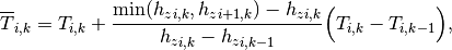
where  is the height of T-cells, the horizontal gradient is
computed as
is the height of T-cells, the horizontal gradient is
computed as 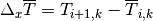 , as shown in Figure5.4 . This approach
seems to be correct but it does not guarantee the negative definiteness
of tracer variance: for example, for the Laplacian horizontal mixing,
, as shown in Figure5.4 . This approach
seems to be correct but it does not guarantee the negative definiteness
of tracer variance: for example, for the Laplacian horizontal mixing,
(113)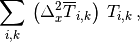
is not sign-definite! A correct approach is to work with the functional which can be written as
(114)¶![{\cal G}[T]=-\frac{1}{2}\sum\frac{h_yh_z}{h_x}\Big (\Delta_x
{\overline T}\Big)^2\,,](../_images/math/1515d7008a913d06dbd23dfd1bbe2a481433a950.png)
where  and
and  are the horizontal grid sizes of
T-cells in the and directions, respectively. Taking
the functional derivative leads to the following discretization for the
horizontal Laplacian diffusion:
are the horizontal grid sizes of
T-cells in the and directions, respectively. Taking
the functional derivative leads to the following discretization for the
horizontal Laplacian diffusion:
![\begin{aligned}
% \frac{\delta {\cal G}}{\delta T} =
dV_T\,D[T]= \Delta_x\left [\,\left(\frac{h_yh_z}{h_x}\right )\,
{\overline \kappa}^x\, \Delta_x \overline T\,\,\right ]
+ \Delta_x\left [\left (\frac{h_y}{h_x}\right )
\Delta_z\left (\gamma h_z{\overline \kappa}^x\Delta_x
\overline T\,\right )\,\right ]\nonumber\end{aligned}](../_images/math/7e061b0d0d57f5a9a8d64eae449457b03e24fd82.png)
(115)¶![\begin{aligned}
\hspace{2cm}
+\Delta_y\left [\,\left(\frac{h_xh_z}{h_y}\right )\,
{\overline \kappa}^y\, \Delta_y\overline T\,\,\right ]
+ \Delta_y\left [\left (\frac{h_x}{h_y}\right )
\Delta_z\left (\gamma h_z{\overline \kappa}^y\Delta_y
\overline T\,\right )\,\right ]\,.
\end{aligned}](../_images/math/4e4a02937a28ec10daae4beccd147dcc6b17a056.png)
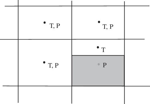
Figure 5.3: Pressure and tracer points in the - plane
above partially-filled bottom cells.
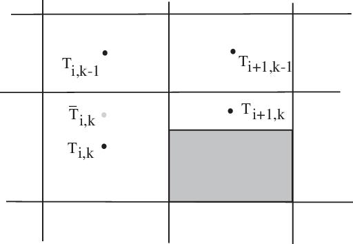
Figure 5.4: Interpolating tracer points to the same level before taking horizontal derivatives.
Since the correct discretization even for the simple Laplacian mixing is too complicated and thus expensive to employ, we have made the partial-bottom-cell implementation in POP in the following ways: (1) we leave the pressure points at the same z-levels which introduces no pressure error and guarantees energetic consistency. Even though some pressure points are underneath the ocean floor, the pressure is computed by extrapolating tracers, therefore density, to pressure points. (2) when we compute the tracer gradients in diffusion operators, we make no interpolation for tracers. This approach introduces spurious diffusion errors but guarantees at least the sign-definite tracer variances, which has been given up in other OGCMs. Our test results show the error introduced by the second approach is so small that we can avoid any complication involving the interpolation.
6.2.2.1. Discretization
After reading the height of bottom T-cells, POP uses two additional
three-dimensional arrays for the thickness of T-cells,
 , and the thickness of
  -cells defined
as
-cells defined
as
(116)
Due to these variable cell heights, the spatial discretizations described in Sec. Spatial Discretization need to be modified as shown in the following.
Tracer Advection:
(117)
where  ,
,
 ,
,  ,
and the vertical velocity at bottom
,
and the vertical velocity at bottom  -cells is found
as
-cells is found
as
(118)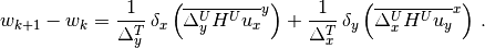
Laplacian Horizontal Tracer Diffusion:
(119)
where =HTN, =HTE, and
(120)
Vertical Tracer Diffusion:
(121)¶![{\cal D}_V(\varphi) = \frac{1}{H^T}\left [
\frac{\kappa_{k+\frac{1}{2}}(\varphi_{k+1}-\varphi_k)}
{({H^T}_{k+1}+{H^T}_{k})/2} -
\frac{\kappa_{k-\frac{1}{2}}(\varphi_k-\varphi_{k-1})}
{(H^T_{k}+H^T_{k-1})/2}\right ].](../_images/math/424aa0ea2c590f3d1720f48a7c5685a58e1705cd.png)
Momentum Advection:
(122)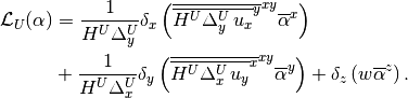
Laplacian Horizontal Friction:
(123)¶![\begin{aligned}
{\cal D}_H({\bf u}) & = \frac{1}{H^U\Delta_y^U}\delta_x\left(
\overline{A_M}^x\Delta_y^i\Delta_z^i\delta_x{\bf u}\right )
+\frac{1}{H^U \Delta_x^U}\delta_y\left(
\overline{A_M}^y\Delta_x^j\Delta_z^j\delta_y{\bf u}\right )
\nonumber \\
& - \frac{A_M}{H^U\Delta_x^U\Delta_y^U}
\left[\,\overline{\frac{\Delta_y^i (H^U-\Delta_z^i)}{\Delta_x}^x}
+\overline{\frac{\Delta_x^j (H^U-\Delta_z^i)}{\Delta_y}^y}
\right ]{\bf u},
\end{aligned}](../_images/math/ff818a69a766d3d94d3edb86705f3ca0fa31feca.png)
where =HTN, =HTE,
 =HUS,
=HUS,  =HUW, and
(124)
The last term of (123) is the drag due to the no-slip boundary condition at lateral boundaries. Metric terms in the momentum advection and horizontal friction remain unaffected by partial bottom cells.
Vertical Friction:
(125)¶![{\cal D}_V({\bf u}) = \frac{1}{H^U}\left [
\frac{\kappa_{k+\frac{1}{2}}({\bf u}_{k+1}-{\bf u}_k)}
{(H^U_{k+1}+H^U_{k})/2}-
\frac{\kappa_{k-\frac{1}{2}}({\bf u}_k-{\bf u}_{k-1})}
{(H^U_{k}+H^U_{k-1})/2}\right ].](../_images/math/6515978537cb07709827f09a7705bc35b8795efc.png)
Hydrostatic Pressure: Since we leave the pressure points at the middle of full cells, the hydrostatic pressure is computed in the same way as for the full-cell case.
Biharmonic Horizontal Diffusion and Friction: The same operations for
the Laplacian diffusion and friction given by (119) and (123)
for and , respectively, are applied
twice.
Isopycnal Diffusion:
(126)¶![\begin{aligned}
{\cal D}_H (\varphi) & =
\frac{1}{H^T\Delta_y^T}\delta_x
\left[{\Delta_y}\left (\overline{H^T{\overline\kappa}^{z}}^x
\delta_x\varphi -
\overline{H^T \overline{\kappa S_x\delta_z\varphi}^{z}}^x
\right )\right ] \\
& - \frac{1}{\Delta_x^T \Delta_y^T}
\delta_z\left[\frac{1}{\overline {H^T}^z}\left (\overline{H^T
\overline{{\Delta_x^j}{\Delta_y}
\kappa S_x \delta_x\varphi}^x}^z - \overline{H^T\overline{
{\Delta_x^j}{\Delta_y} \kappa S_x^2}^x}^z
\delta_z \varphi \right )\right ]
\nonumber \\
& + \frac{1}{H^T\Delta_x^T}\delta_y
\left[{\Delta_x}\left (\overline{H^T{\overline\kappa}^{z}}^y
\delta_y\varphi -
\overline{H^T\overline {\kappa S_y
\delta_z\varphi}^{z}}^y\right )\right ]
\nonumber \\
& - \frac{1}{\Delta_x^T \Delta_y^T}
\delta_z\left[\frac{1}{\overline {H^T}^z}\left (\overline{H^T
\overline{{\Delta_x}{\Delta_y^i}
\kappa S_y \delta_y\varphi}^y}^z - \overline{H^T\overline{
{\Delta_x}{\Delta_y^i} \kappa S_y^2}^y}^z
\delta_z \varphi \right )\right ],
\nonumber\end{aligned}](../_images/math/dc3a05e2b9c3b4b2c09609fdf811c4c84ea68f9d.png)
where =HTN, =HTE,
=HUS, =HUW,
 , and
, and
 . In (126), for example, in the
 -plane, in the two quarter cells in either
the east or west direction of T-cells right next to any partial cell is
reduced to
-plane, in the two quarter cells in either
the east or west direction of T-cells right next to any partial cell is
reduced to
(127)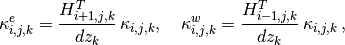
where is the full-cell height. Similar reductions are made
for in the  -plane, too. Also
in the lower half of T-cells right above any partial cells and
in the upper half of any partial cells are modified to
-plane, too. Also
in the lower half of T-cells right above any partial cells and
in the upper half of any partial cells are modified to
(128)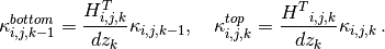
Remember that at the lower half of bottom T-cells is set
to zero.
Anisotropic Viscosity:
(129)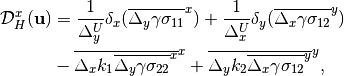
(130)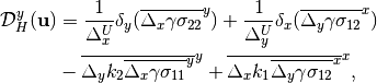
where =HTN, =HTE,  at four quarter cells at the centered U-cell and
  ’s are
defined in two quarter cells adjacent to the U-cell in the east, west,
north and south directions as
’s are
defined in two quarter cells adjacent to the U-cell in the east, west,
north and south directions as
(131)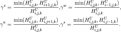
Due to no-slip boundary conditions imposed at lateral boundaries, the
velocity gradients to compute the stress tensor  are
re-defined as
are
re-defined as
(132)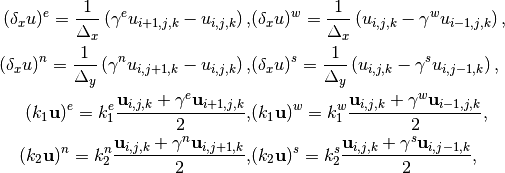
where  ,
,  ,
,  and
and  are
the metric terms defined on the east, west, north and south faces.
are
the metric terms defined on the east, west, north and south faces.
7. Advection
POP supports a few advection schemes, primarily for tracers where conservation and monotonicity requirements are stronger. While basic centered schemes for tracers and advection are described in Chapter Spatial Discretization, this chapter describes other advection schemes implemented in POP.
7.1. Third-Order Upwind Advection
Third-order upwind schemes and variants of this scheme were introduced by Leonard (1979a). Our implementation of third-order upwinding simply involves the substitution of three-point interpolation for the two-point centered average in the determination of the tracer value at cell faces, and remains in leapfrog temporal implementation.
It should be noted that improved temporal implementations have been explored in Farrow and Stevens (1995), where they apply a predictor-corrector sequence, and in Holland, Bryan, and Chow (1998), where in addition to documenting our implementation they also describe a reorganization of terms into two groups, one of which is entirely centered in space, the other having a dissipative form.
The finite-difference expression for the advection of tracers is
(133)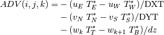
where :math:` {u}_W, {u}_E, {v}_S, {v}_N` are the T-grid cell face
centered velocity components and the directions  and
and
 are with respect to the logical coordinates.
(134)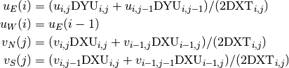
and the  quantities are the cell face centered tracer
concentration at the east, west, north, south, top, and bottom faces. In
the standard second-order scheme of POP, these are taken as the
arithmetic average of the tracer concentrations in adjacent cells, e.g.,
quantities are the cell face centered tracer
concentration at the east, west, north, south, top, and bottom faces. In
the standard second-order scheme of POP, these are taken as the
arithmetic average of the tracer concentrations in adjacent cells, e.g.,
(135)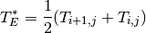
The third point included in the three-point interpolation is taken to be in the upwind direction,
(136)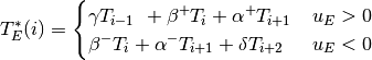
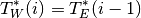
where the coefficients  are given
by
are given
by
(137)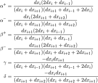
where  and the -index is suppressed for
clarity. The interface tracer values
and the -index is suppressed for
clarity. The interface tracer values  , and
, and
 are obtained in an analogous manner.
7.2. Flux-Limited Lax-Wendroff Algorithm
A flux-limited version of the second-order Lax-Wendroff advection scheme has been introduced into POP. The scheme is designed to reduce, but not completely eliminate, the production and amplification of artificial extrema. The artificial extrema are not completely eliminated because the flux limiter is not a true multidimensional limiter. The scheme is constructed by combining a one-dimensional flux-limited scheme with a dimensional splitting technique. We describe in order: time stepping, the non-flux limited version of the one dimensional scheme, the flux limiter, the dimensional splitting technique, and how boundary conditions are handled.
The advection schemes currently available in POP, centered and
third-order upwind, use leap-frog time stepping. That is, when computing
the tracer tendency between time levels and the
advective operator  is applied to the tracer
at time level . However, flux-limited advection
schemes are generally designed for forward-in-time time stepping. So
this scheme applies the advective operator to the tracer
time level . Note that velocities are still from time level
and thus are time-centered.
is applied to the tracer
at time level . However, flux-limited advection
schemes are generally designed for forward-in-time time stepping. So
this scheme applies the advective operator to the tracer
time level . Note that velocities are still from time level
and thus are time-centered.
The advection equation in one dimension, in advective form, is
(138)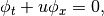
where is the component of the velocity in the dimension under
consideration. We rewrite (138) as
(139)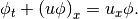
While we assume that  , we do not assume
the velocity to be divergence-free in one dimension. Because of this,
(138) and (139) do not
necessarily conserve total tracer content. Conservation of total tracer
content will later be recovered with the splitting scheme described
below.
, we do not assume
the velocity to be divergence-free in one dimension. Because of this,
(138) and (139) do not
necessarily conserve total tracer content. Conservation of total tracer
content will later be recovered with the splitting scheme described
below.
For our description of the non-flux limited one-dimensional scheme, we
temporarily change notation from that used elsewhere in this manual. We
consider a one dimensional grid where the th interval of the
grid is denoted  . Its width is
  , its
midpoint is
, its
midpoint is  , and its left and right endpoints are
 and
and  respectively. Thus, we have
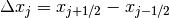 . Additionally, we define
 . The
advection scheme under consideration discretizes
(139) as
. The
advection scheme under consideration discretizes
(139) as
(140)
where super- and sub-scripts indicate time and space indices
respectively and is the time step.  ,
the advective flux of through , is given
by
,
the advective flux of through , is given
by
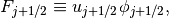
where  is an approximation to the average value of
at over
is an approximation to the average value of
at over
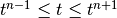 . Since does not
represent at a particular time level, we do not denote a
time level in a superscript. is constructed by
. Since does not
represent at a particular time level, we do not denote a
time level in a superscript. is constructed by
- approximating
 with a linear fit
  ,
, - advecting exactly with velocity
 ,
, - taking to be the average value of the advected at over .
The linear fit is constructed by equating ’s
average values over intervals  near to
 for
for  . That is, satisfies the constraints
(141)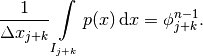
When the constructed is advected and averaged at
 over , the result
is
over , the result
is
(142)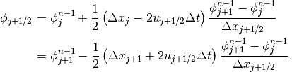
This is the familiar Lax-Wendroff scheme in a form that is appropriate for a stretched grid. We present the different forms of the same expression in anticipation of the application of flux limiters.
The above description assumes that the velocity is specified at interval
boundaries. This leads to a natural implementation in the
multidimensional setting when normal velocities are specified at
midpoints of tracer cell faces, as is done with Arakawa C-grids (Arakawa
and Lamb 1977). However, POP utilizes an Arakawa B-grid, where
velocities are specified at tracer cell corners. Since the
one-dimensional scheme use the face velocity for the tracer face value
construction, e.g. (142), it is necessary to
compute a face velocity from the B-grid corner velocities. The normal
velocity for the east face of the tracer cell is computed as
(143)
where  ,
,
 is the length of the east face, and
 and
and  are the zonal
velocities at the north-east and south-east corners respectively. We
note that (143) requires adjustment if
POP is configured with partial bottom cells and that a formula analogous
to (143) holds for
are the zonal
velocities at the north-east and south-east corners respectively. We
note that (143) requires adjustment if
POP is configured with partial bottom cells and that a formula analogous
to (143) holds for
 .
.
In one dimension, we employ a flux limiter that is based on the work of
Hundsdorfer and Trompert (1994), noting that the flux limiter presented
there is in fact equivalent to the ULTIMATE flux limiter of Leonard
(1979b). Solutions of (138) are constant along
characteristics, which implies that local extrema are not created or
amplified. The purpose of the flux limiter is to constrain the
discretization to have this property as well. This is done by modifying,
as necessary, the advective flux . In order to simplify
the presentation, we initially assume  . We write
as
. We write
as
(144)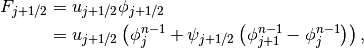
where  is to be determined. A priori, we will impose
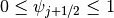 in order to avoid extrapolation in
the construction of . We seek further constraints on
that will ensure
in order to avoid extrapolation in
the construction of . We seek further constraints on
that will ensure
(145)
Note that constraints on are ensuring extrema
constraints on the interval that is upwind of and that
these extrema constraints are expressed in terms of upwind values. Given
this form for ,
(140) becomes
(146)¶![\begin{split}
\phi^{n+1}_{j} & = \phi^{n-1}_{j} - \frac{2 \Delta t}{\Delta x_{j}} \Big[
\mathbin{\phantom{-}} u_{j-1/2} \phi^{n-1}_{j\phantom{-1}}
+ u_{j+1/2} \psi_{j+1/2}
\left( \phi^{n-1}_{j+1} - \phi^{n-1}_{j} \right) \\
& \mathrel{\phantom{=}}
\phantom{\phi^{n-1}_{j} - \frac{2 \Delta t}{\Delta x_{j}} \Big[}
- u_{j-1/2} \phi^{n-1}_{j-1} - u_{j-1/2} \psi_{j-1/2}
\left( \phi^{n-1}_{j} - \phi^{n-1}_{j-1} \right) \Big]
\end{split}](../_images/math/d40739c090d7597b85f81f1e4d1b5337a90d9560.png)
We now consider two very specific cases and then the more general third case:
: 
In this case, (146) reduces to
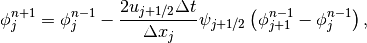
and (145) reduces to
 . Together, these imply
 .
.
: 
In this case, (146) reduces to
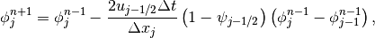
so there is no constraint on .
: 
Letting
 ,
(146) becomes
,
(146) becomes
![\begin{split}
\phi^{n+1}_{j} & = \bigg[ 1 - \frac{2 \Delta t}{\Delta x_{j}}
\left( u_{j-1/2} \left( 1 - \psi_{j-1/2} \right)
+ u_{j+1/2} \psi_{j+1/2} / \theta_{j} \right)
\bigg] \phi^{n-1}_{j} \\
& \mathrel{\phantom{=}}\phantom{\bigg[ 1}
+ \frac{2 \Delta t}{\Delta x_{j}}
\left( u_{j-1/2} \left( 1 - \psi_{j-1/2} \right)
+ u_{j+1/2} \psi_{j+1/2} / \theta_{j} \right)
\phi^{n-1}_{j-1}. \nonumber
\end{split}](../_images/math/2ad10f2fb71b89c7d78b0568166604fa5106c9a3.png)
This expresses  as a linear combination of
 and
and  where the weights
sum to 1. Given such a representation,
(145) is equivalent to requiring
the weights to be between 0 and 1. Thus,
(145) is equivalent to
where the weights
sum to 1. Given such a representation,
(145) is equivalent to requiring
the weights to be between 0 and 1. Thus,
(145) is equivalent to
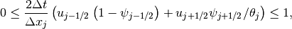
which in turn is equivalent to
(147)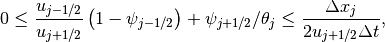
where we have used the assumption  . We now suppose
that
. We now suppose
that
(148)
where  is to be determined, and
 is the value of that
corresponds to the non-flux limited advection scheme. Then
is the value of that
corresponds to the non-flux limited advection scheme. Then

It follows that

Comparing this to (147), we see that (147), and thus (145), will be ensured if
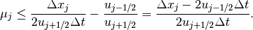
In the above presentation we assumed that . The velocities
used in the analysis were and the velocity in the
upwind direction,  . With this in mind, the remaining
cases to consider are
. With this in mind, the remaining
cases to consider are  , and
, and
 , and
, and  and
and  .
The last velocity sign pair is merely a shift by +1 of the
indices from the second pair, so it is not necessary to separately
consider this case. We note that the converging velocity pair
and
.
The last velocity sign pair is merely a shift by +1 of the
indices from the second pair, so it is not necessary to separately
consider this case. We note that the converging velocity pair
and  does not arise in our
analysis because when , the analysis depends on
does not arise in our
analysis because when , the analysis depends on
 .
.
We now consider the case where . In order to maintain the
notion that smaller values of correspond to greater
diffusion, (144) is replaced with
(149)
In order to maintain the notion that constraints on
are ensuring extrema constraints on the upwind interval,
(145) is replaced with
(150)
Assuming  , we find, with
similar algebra, that
(150)
will be satisfied if
, we find, with
similar algebra, that
(150)
will be satisfied if
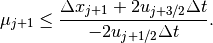
We finally consider the case where and
. In this case, we use
(144) for and
(149) for
 . Then (140) becomes
![\begin{split}
\phi^{n+1}_{j} & = \phi^{n-1}_{j} - \frac{2 \Delta t}{\Delta x_{j}} \Big[
\mathbin{\phantom{+}}
u_{j+1/2} \psi_{j+1/2} \left( \phi^{n-1}_{j+1} - \phi^{n-1}_{j} \right) \\
& \mathrel{\phantom{=}}
\phantom{\phi^{n-1}_{j} - \frac{2 \Delta t}{\Delta x_{j}} \Big[}
+ u_{j-1/2} \psi_{j-1/2} \left( \phi^{n-1}_{j} - \phi^{n-1}_{j-1} \right)
\Big].
\end{split}](../_images/math/e7bdfd9dd1e99c2723424ea79cf28cde06afcf19.png)
Since is upwind of both and
, we use constraints on both and
 to ensure extrema constraints on
. Since there are no points upwind of
, the extrema constraints reduce to
to ensure extrema constraints on
. Since there are no points upwind of
, the extrema constraints reduce to
 . This can only be satisfied if
(151)
We now consider two very specific cases and then the more general third case:
:
Then we must have . The value of
 is irrelevant.
: 
Then we must have  . The value of
 is irrelevant.
:
Then (151) can be divided by
 to obtain
(152)
If  , the only solution that satisfies
 is
is 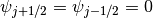 . If
. If  ,
we choose the largest values of and
that satisfy (152),
,
we choose the largest values of and
that satisfy (152),
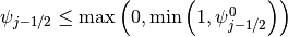 ,
and
,
and 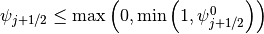 .
We do this by setting
.
We do this by setting
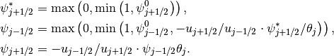
The dimensional splitting technique follows the technique described in
section 2.17.4 of Adcroft et al. (2005). In our implementation of this
technique, (140) and
(144) are applied sequentially in the
, , and directions. Each application of this
pair of equations uses the results from the previous application, except
for the last term of (140), where we
use  in each iteration. Using for
this term in each iteration leads to conservation of total tracer
content, assuming as we do that the velocity field is divergence free.
Our choice of the ordering of dimensions is based on simplifying the
implementation. We tested alternating the dimension order in simulations
of the Stommel gyre test problem of Hecht, Holland, and Rasch (1995) and
did not find a meaningful benefit, so we do not vary the dimension order
in the three-dimensional setting.
in each iteration. Using for
this term in each iteration leads to conservation of total tracer
content, assuming as we do that the velocity field is divergence free.
Our choice of the ordering of dimensions is based on simplifying the
implementation. We tested alternating the dimension order in simulations
of the Stommel gyre test problem of Hecht, Holland, and Rasch (1995) and
did not find a meaningful benefit, so we do not vary the dimension order
in the three-dimensional setting.
The flux limiter extends the discrete domain of dependence of
Lax-Wendroff in the upstream direction, potentially beyond lateral
boundaries. For example, consider the situation where we are computing
the ’zonal’ flux at , , and there is
a solid boundary at .
Using (144) for and
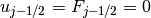 in
(140) yields
in
(140) yields
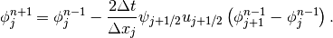
Since is upwind of , we use constraints
on to ensure extrema constraints on
. Since there are no points upwind of
in the direction under consideration, the extrema
constraints reduce to . This can
only be satisfied if . Examining
(148), this can be achieved by using
 , which is equivalent to using a fictitious
 . In other words, we use a zero
Neumann boundary condition at no-flow boundaries.
. In other words, we use a zero
Neumann boundary condition at no-flow boundaries.
8. Sub-grid Scale Mixing Parameterizations
8.1. Horizontal Tracer Diffusion
8.1.1. Laplacian Horizontal Diffusivity
The spatial discretization of the standard Laplacian horizontal tracer
diffusion with a spatially varying tracer diffusivity  is
described in Sec. Horizontal Tracer Diffusion.
is
described in Sec. Horizontal Tracer Diffusion.
8.1.2. Biharmonic Horizontal Diffusivity
Biharmonic horizontal tracer diffusion is implemented by applying the Laplacian operator (41) twice. Specifically,
(153)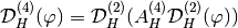
where the superscripts (4) and (2) refer to biharmonic and harmonic
(Laplacian) operators, and  is given by
(41) with
is given by
(41) with  .
.  is the biharmonic
diffusivity, which may be spatially varying, and should be negative for
positive-definite diffusion. Here the biharmonic diffusivity is
sandwiched between the two applications of the Laplacian operator. An
alternate approach (not implemented in the code), following Griffies and
Hallberg (2000), is to include the square-root of
is the biharmonic
diffusivity, which may be spatially varying, and should be negative for
positive-definite diffusion. Here the biharmonic diffusivity is
sandwiched between the two applications of the Laplacian operator. An
alternate approach (not implemented in the code), following Griffies and
Hallberg (2000), is to include the square-root of  inside
the second derivative of each operator.
inside
the second derivative of each operator.
8.1.3. The Gent-McWilliams Parameterization
The transport equation of tracer is given by
(154)
where the bolus velocity induced by mesoscale eddies is parameterized, from Gent and McWilliams (1990), as
(155)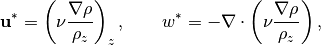
where  is a thickness diffusivity and subscripts
 on and tracers denote partial
derivatives with respect to those variables (this convention will be
followed below). The Redi isoneutral diffusion operator (Redi 1982) for
small slope can be written as
on and tracers denote partial
derivatives with respect to those variables (this convention will be
followed below). The Redi isoneutral diffusion operator (Redi 1982) for
small slope can be written as
(156)
where the subscript 3 indicates the three-dimensional gradient or
divergence, i.e.,
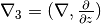 . The symmetric
tensor K is defined as
. The symmetric
tensor K is defined as
(157)
This tensor describes along-isopycnal diffusion that is isotropic in
the two horizontal dimensions. The general anisotropic form of (157) is
given in Smith (1999). The isopycnal diffusivity  is in
general a function of space and time, and a parameterization for
variable will be described at the end of this section.
In POP, we write the bolus velocity in the skew-flux form (Griffies
1998):
is in
general a function of space and time, and a parameterization for
variable will be described at the end of this section.
In POP, we write the bolus velocity in the skew-flux form (Griffies
1998):
(158)
where we have used :math:` nabla_3cdot {bf u}_3^*=0`. The subscript
3 on the velocity indicates the three-dimensional velocity, i.e.,
 . The antisymmetric tensor B
is given by
. The antisymmetric tensor B
is given by
(159)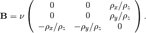
By substituting (159), the transport equation (154) can be written
(160)
With a nonlinear equation of state, the isopycnal slopes
 that appear in
(157) and (159) should be replaced with slopes along the local neutral
surfaces (McDougall 1987), which are given by:
that appear in
(157) and (159) should be replaced with slopes along the local neutral
surfaces (McDougall 1987), which are given by:
(161)
with a similar definition for  . Here
 and
and
 , where
and are the model potential temperature and salinity, and
, where
and are the model potential temperature and salinity, and
 is the potential density referenced to the local pressure
(or depth).
is the potential density referenced to the local pressure
(or depth).
8.1.3.1. Discretization of the Diffusion Operator
The functional formalism for deriving positive-definite diffusive operators in ocean models was originally used to implement the Gent-McWilliams parameterization in POP. Later, a collaboration between GFDL and LANL led to an improved implementation that is described in Griffies et al. (1998). The main change in the new formulation is to discretize the neutral slopes (161) in a particular way that avoids exciting a nonlinear instability.
The discrete functional formalism is based on the property of the
continuous dissipation operator (160) that it can be expressed as the
functional derivative of the integral of a positive-definite functional
 :
:
(162)¶![\begin{aligned}
{\cal G}[\varphi] &= \frac{1}{2}\int dV
(\nabla_3\varphi)\cdot{\bf K}\cdot(\nabla_3\varphi) \nonumber \\
&= \frac{1}{2} \int dV \kappa_I
\left[(\varphi_x + L_x\varphi_z)^2
+ (\varphi_y + L_y\varphi_z)^2\right]
\\
R(\varphi) &= -\frac{\delta}{\delta \varphi} {\cal G}[\varphi]
\end{aligned}](../_images/math/1e1325799bb92aa7b4ed9565e753711641275a3b.png)
where  denotes a functional derivative. That is,
is a functional whose derivative with respect to a
tracer field at a given point in space yields the isoneutral diffusive
operator at that point. Note that, as a consequence of the
assumption of isotropic diffusion (157), the 3-D functional splits into
two terms which are effectively 2-D, one in the
denotes a functional derivative. That is,
is a functional whose derivative with respect to a
tracer field at a given point in space yields the isoneutral diffusive
operator at that point. Note that, as a consequence of the
assumption of isotropic diffusion (157), the 3-D functional splits into
two terms which are effectively 2-D, one in the  plane and
one in the
plane and
one in the  plane.
The procedure for deriving the discrete operator is to first discretize
the functional and then take its derivatives with respect to the tracer
field at a given point on the computational grid; this yields the
positive-definite diffusion operator at that point. In order to
discretize the functional on the POP grid, we need to define all the
quantities appearing in within each cell. Because
gradients involve differences across cell faces, it is convenient to
subdivide each T-cell into four subcells, as shown in
Figure7.1 , which shows a central T-cell, its four interior
subcells, and the eight surrounding subcells that contribute to the
friction operator when the discrete functional derivative is taken with
respect to the tracer value at the central point. A unique value of the
tracer gradients and isoneutral slopes can be assigned to each subcell,
and from these the complete discrete functional can be
constructed and summed over the grid. Associated with each subcell is
the set of its three nearest points (known as the “triad” of points
associated with that subcell), namely, the central point of the full
cell to which it belongs, and the two nearest points in the horizontal
and vertical directions. For example, the triad associated with the
subcell in Figure7.1 labeled ( ) is the set of
points labeled (
) is the set of
points labeled ( ), (), (
 ). All the
derivatives of the tracer fields needed to construct the functional in a
given subcell only involve the tracer values at its triad points. For
example, the and derivatives of in
the subcell labeled (), are given by
). All the
derivatives of the tracer fields needed to construct the functional in a
given subcell only involve the tracer values at its triad points. For
example, the and derivatives of in
the subcell labeled (), are given by
 and
and
 , where
and are defined in each subcell as the distances
between the central point () and the other two triad points in
the and directions, respectively. Similarly, the
derivatives in the subcell labeled (
, where
and are defined in each subcell as the distances
between the central point () and the other two triad points in
the and directions, respectively. Similarly, the
derivatives in the subcell labeled ( ) are given by
 and
and
 . The
diffusion coefficient is assumed to have a constant value across all
four subcells within a given full cell, but can vary from full-cell to
full cell.
. The
diffusion coefficient is assumed to have a constant value across all
four subcells within a given full cell, but can vary from full-cell to
full cell.
Using these definitions of the quantities in each subcell appearing in (162), it can be written in the discrete form:
(163)¶![{\cal G}[\varphi] = \frac{1}{2}\sum_{ij}\sum_{n=1}^4
(\kappa_I)_{ij} V_{ijn} [(\varphi_x + L_x\varphi_z)^2
+ (\varphi_y + L_y\varphi_z)^2]](../_images/math/74a7b8c74c541bee9f8333a475f9d15ef7cd7e65.png)
where subscripts  run over all full cells, and subscripts
over subcells within a given full cell.
run over all full cells, and subscripts
over subcells within a given full cell.
 is the subcell volume (where
is the full cell width centered at the same point as
, and note that the height of each subcell is taken to be
half its full-cell height
is the subcell volume (where
is the full cell width centered at the same point as
, and note that the height of each subcell is taken to be
half its full-cell height  .)
.)
The diffusion operator is then given by the derivative of the discrete
functional with respect to the velocity at a given point
 :
:
(164)¶![R_{i'j'} = -\frac{1}{V^T_{i'j'}}
\frac{\partial}{\partial\varphi_{i'j'}}
G[\varphi]](../_images/math/0a545a16a9ee575903d1a4a47f4ed28d8c225fbd.png)
where  full-cell volume of cell
(), and
full-cell volume of cell
(), and  is the full-cell area. (Note: in
the code
is the full-cell area. (Note: in
the code  , which is not exactly equal to the
sum of the four subcell areas given above, however, the difference is
small and is absorbed in an overall normalization factor.) When taking
the derivative with respect to at the central point,
only those subcells in the full functional whose triad points contain
the central point will contribute to the derivative, and these are just
the 12 subcells shown in Figure7.1 . It is straightforward
to take the derivative in (164) in these 12 subcells and
assemble the results into a compact form for the diffusion operator. The
result is:
, which is not exactly equal to the
sum of the four subcell areas given above, however, the difference is
small and is absorbed in an overall normalization factor.) When taking
the derivative with respect to at the central point,
only those subcells in the full functional whose triad points contain
the central point will contribute to the derivative, and these are just
the 12 subcells shown in Figure7.1 . It is straightforward
to take the derivative in (164) in these 12 subcells and
assemble the results into a compact form for the diffusion operator. The
result is:
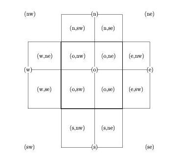
Figure 7.1: The discretization of the part of the isoneutral
diffusion functional is accomplished by subdividing each T-cell
(shown bounded by thick lines) into four subcells. The central tracer
point (T-point) is denoted by “(o)” and the surrounding T-points by
“(n)”, “(s)”, “(ne)”, etc. (this is for notation only, points “(n)”
and “(s)” are displaced in the vertical direction.) The four subcells
surrounding the central point are labeled “(o,ne)”, “(o,nw)”, etc.,
and the subcells surrounding the T-cell to the east are labeled
“(e,nw)”, etc. Within each subcell a unique value is defined for all
quantities (e.g., the gradients and slope factors appearing in
(162) that are needed to evaluate the functional. Only the
twelve subcells shown contribute to the friction operator at the
central point (see text). (Note: this figure shows a case where the
fundamental grid is constructed with U-points in the exact middle of
T-cells in a grid with variable horizontal spacing. More commonly
T-points are located at the exact center of U-cells. This choice is
made during grid generation and is only determined in the code
through the input grid file.) This figure can also be used for
constructing the anisotropic dissipation functional (see
Sec. Anisotropic Horizontal Viscosity) where the central point represents a U-point.
(165)
Here overbars with superscripts , , etc., denote sums
over the four subcells surrounding the east, west, etc., faces of the
central full cell. In computing the slopes  and
given by (161) it is important that the coefficients
and
given by (161) it is important that the coefficients
 and
and  be evaluated at the pressure
corresponding to the level of the central point of the triad in a given
subcell (Griffies et al. 1998); this avoids exciting the nonlinear
instability mentioned above. No-flux boundary conditions on the tracers
are implemented by setting
be evaluated at the pressure
corresponding to the level of the central point of the triad in a given
subcell (Griffies et al. 1998); this avoids exciting the nonlinear
instability mentioned above. No-flux boundary conditions on the tracers
are implemented by setting  in all subcells adjacent
to lateral and bottom boundaries. There is no way to derive the bolus
transport term in (160) and (159) from a functional like the diffusive
term, but the bolus term in (160) involves terms proportional to the
off-diagonal terms in the diffusion tensor, and these are discretized in
the same way. Thus we find for the full skew flux
(
in all subcells adjacent
to lateral and bottom boundaries. There is no way to derive the bolus
transport term in (160) and (159) from a functional like the diffusive
term, but the bolus term in (160) involves terms proportional to the
off-diagonal terms in the diffusion tensor, and these are discretized in
the same way. Thus we find for the full skew flux
( in (160))
(166)¶![\begin{aligned}
V^{T}_{ij}\overline{R}_{ij}(\varphi) &=
\overline{(V/h_x)[\kappa_I\varphi_x + (\kappa_I-\nu)L_x\varphi_z]}^e
\nonumber \\
&- \overline{(V/h_x)[\kappa_I\varphi_x + (\kappa_I-\nu)L_x\varphi_z]}^w
\nonumber \\
&+ \overline{(V/h_z)[(\kappa_I+\nu)L_x\varphi_x +
\kappa_I L_x^2\varphi_z]}^n
\nonumber \\
&- \overline{(V/h_z)[(\kappa_I+\nu)L_x\varphi_x +
\kappa_I L_x^2\varphi_z)}^s
\nonumber \\
&+ \ \mathrm{similar\ terms\ with}\ x\ \mathrm{replaced\ by}
\ y\ \mathrm{everywhere.}
\end{aligned}](../_images/math/114e7d19f33851f11ecd4bb2d648a5f68417c916.png)
If the tracer and thickness diffusion coefficients are chosen equal
( ), then the second terms in brackets in the first
line of (166) vanish and need not be computed. (Note: in
the code, the above formulae are evaluated using the slope functions
), then the second terms in brackets in the first
line of (166) vanish and need not be computed. (Note: in
the code, the above formulae are evaluated using the slope functions
 ,
,
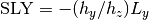 , and the differences
 , etc.) Finally, it should be
noted that the last terms in (166) involving
, etc.) Finally, it should be
noted that the last terms in (166) involving
 (and
(and  ) are separated and treated implicitly,
because the effective viscous coefficient can be large enough to violate
explicit CFL conditions (Cox 1987). These terms can be written
) are separated and treated implicitly,
because the effective viscous coefficient can be large enough to violate
explicit CFL conditions (Cox 1987). These terms can be written
(167)
and the last line gives  on the top of the T-cell.
is then added to the vertical diffusivity
in (42) and the vertical diffusion is solved implicitly. For
this reason implicit vertical mixing must be used with the
Gent-McWilliams parameterization. One of the design features of the
diffusive operator is that with a linear equation of state it should be
zero when applied to
on the top of the T-cell.
is then added to the vertical diffusivity
in (42) and the vertical diffusion is solved implicitly. For
this reason implicit vertical mixing must be used with the
Gent-McWilliams parameterization. One of the design features of the
diffusive operator is that with a linear equation of state it should be
zero when applied to  . This condition is violated
when the above term is treated implicitly while the remaining terms are
treated explicitly, but in practice this leads to a very small error and
is ignored.
. This condition is violated
when the above term is treated implicitly while the remaining terms are
treated explicitly, but in practice this leads to a very small error and
is ignored.
Two tapering functions are often applied to the GM coefficient
and the Redi mixing coefficient . The first
is for physical reasons and reduces the GM coefficient in the upper
boundary layer, see Large et al. (1997). Here the ocean is not nearly
adiabatic, and so the GM parameterization does not apply; instead the
isopycnals tend to become more vertical because of the strong vertical
mixing in the upper boundary layer. The tapering occurs where the depth
is less than the local isopycnal slope multiplied by the local Rossby
radius  defined by
  with
with
 m/s and is bounded by
 . Two forms for the factor
are in the code, with the second being faster because there is no sine
function.
. Two forms for the factor
are in the code, with the second being faster because there is no sine
function.
tanh option:
(168)¶![f_1 = \frac{1}{2} \Big[1+
\sin\Big(\pi (\min(1, -z/(\vert{\bf L}\vert L_R))-0.5)\Big)\Big]](../_images/math/f33a119484dcce636f1746ef790e53d2ff08583f.png)
else:
(169)
where  . The second
function ensures numerical stability when the isopycnals become too
steep. There are four options to reduce the coefficients
and for
. The second
function ensures numerical stability when the isopycnals become too
steep. There are four options to reduce the coefficients
and for
 , where the maximum
slope allowed can be different for
, where the maximum
slope allowed can be different for  and
and
 . The default values are
 . The first option was described
in Danabasoglu and McWilliams (1995) as
. The first option was described
in Danabasoglu and McWilliams (1995) as
(170)¶![f_2 = \frac{1}{2}
\Big [1-\tanh (10\vert{\bf L}\vert/ S_M^{(\kappa_I,\nu)}-4)\Big ]](../_images/math/73fabc1f9636f34f6f40b3fcc993a3c401eae275.png)
for  ,
,
 . The second option is a faster version without a
tanh function:
. The second option is a faster version without a
tanh function:
(171)¶![f_2 = \frac{1}{2}
\Big [1-\Big(2.5\vert{\bf L}\vert/ S_M^{(\kappa_I,\nu)}-1\Big)
\Big( 4 - \vert 10\vert{\bf L}\vert/ S_M^{(\kappa_I,\nu)}-4\vert\Big)\Big]](../_images/math/5ec84a9088b68dfeb6424d196ee2252e25b1058b.png)
with  for
for
 and
and
 for
for
 .
.
The third option is the clipping option described in Cox (1987) where
the slopes are set to the maximum if they are diagnosed as larger. In
this case, mixing occurs along the maximum allowed slope. This implies
some cross isopycnal mixing when the slopes are steep. The default
values are .
The fourth option is described in Gerdes, Koberle, and Willebrand (1991) and the factor is
(172)
when the slope is larger than the maximum slope. This option and the
first two options retain the adiabatic nature of the parameterization.
When  and
and  , the
code runs much faster because the terms proportional to
, the
code runs much faster because the terms proportional to
 disappear. Because CCSM uses the Near Surface Eddy
Flux Paramaterization described below, no
disappear. Because CCSM uses the Near Surface Eddy
Flux Paramaterization described below, no  function is
needed. For
function is
needed. For  , CCSM uses the second option, but the maximum
slopes allowed are much larger than the default values with
, CCSM uses the second option, but the maximum
slopes allowed are much larger than the default values with
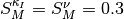 .
.
8.1.3.2. Variable GM Diffusivity
Two options for specifying a variable diffusivity are available. The first follows Visbeck et al. (1997), where it is assumed that
(173)
with a typical value of the constant as 0.13. In (173),
the baroclinic length scale  and the Eady time scale
 are defined as
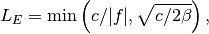
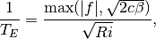
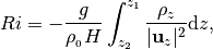
where  is the meridional gradient of the Coriolis
parameter and is the first baroclinic wave speed given by
is the meridional gradient of the Coriolis
parameter and is the first baroclinic wave speed given by
 ,
,
 and
and  . is also
bounded below by the smaller horizontal side of each grid box. In the
code, is set to be bounded by
. is also
bounded below by the smaller horizontal side of each grid box. In the
code, is set to be bounded by
 and
is set to the lower bounding value where the model
depth is less than
and
is set to the lower bounding value where the model
depth is less than  .
.
A second option is meant to parameterize submesoscale eddies. This
option varies the thickness, , and isopycnal diffusivity,
, using a simplified version of the closure of Eden and
Greatbatch (2008) (note that thickness diffusivity and isopycnal
diffusivity are here assumed to be identical). The thickness diffusivity
is given by  , where denotes
an inverse eddy time scale and a constant parameter of order
one.
, where denotes
an inverse eddy time scale and a constant parameter of order
one.  denotes an eddy length scale, which is taken as the
minimum of the local Rossby radius
denotes an eddy length scale, which is taken as the
minimum of the local Rossby radius  and the Rhines scale
 . The latter is estimated from model variables as
 , where
  , while
is given by
, while
is given by
![L_r = min \left[ c_r/|f|, \sqrt{c_r/2\beta}\right]](../_images/math/50db179899b25bd7edbf1a441d44aa6914fcad60.png) where
where
 denotes the first baroclinic Rossby wave speed, which is
calculated approximately by
denotes the first baroclinic Rossby wave speed, which is
calculated approximately by  ,
where
,
where  denotes the local water depth. The inverse eddy time
scale is given by
denotes the local water depth. The inverse eddy time
scale is given by  ,
which is, by the thermal wind relation, for mid-latitudes identical to
the Eady growth rate
,
which is, by the thermal wind relation, for mid-latitudes identical to
the Eady growth rate  , where
 denotes the local
Richardson number. To prevent a singularity for for
denotes the local
Richardson number. To prevent a singularity for for
 we use
  with
with
 which acts effectively as an upper limit for
and consequently for . To prevent a
singularity for the time scale at the equator,
is replaced by
which acts effectively as an upper limit for
and consequently for . To prevent a
singularity for the time scale at the equator,
is replaced by  when computing
. The default values for the parameters of the closure are
set to
when computing
. The default values for the parameters of the closure are
set to  and
and  . More details about the
closure can be found in Eden and Greatbatch (2008) and Eden, Jochum, and
Danabasoglu (2009).
. More details about the
closure can be found in Eden and Greatbatch (2008) and Eden, Jochum, and
Danabasoglu (2009).
8.1.3.3. Near Surface Eddy Flux Parameterization
We have implemented a simplified version of the near-boundary eddy flux parameterization of Ferrari et al. (2008), ((2008), referred to as FMCD08) for the surface boundary in POP. We refer to this scheme as the Near Surface Eddy Flux (NSEF) parameterization. Here, we present a brief summary of its implementation in POP and refer to Danabasoglu, Ferrari, and McWilliams (2008) for further details.
As indicated earlier, the Gent and McWilliams (1990) ((1990), GM90)
parameterization was developed for the quasi-adiabatic interior, and it
is not valid near the boundaries. Therefore, the usual practice is to
taper the effects of parameterized eddy fluxes as the surface (or any
other boundary) is approached (see equations (168) and
(169)). For example, both and are
tapered to zero when the ocean surface is approached using the
taper function in addition to the large slope
taper function using
(174)
the asterisk denotes the tapered values of these diffusivities (Large et al. 1997). This near boundary attenuation of the eddy effects is not physically consistent with observational evidence, particularly near the surface where the diabatic mesoscale fluxes may dominate the mixing. FMCD08 includes the effects of these upper-ocean diabatic fluxes and eliminates the ad-hoc, near-surface taper functions.
The NSEF parameterization requires estimation of two vertical length scales: the boundary layer depth (BLD) and the transition layer thickness (TLT). The BLD can exhibit rapid fluctuations during which mesoscale eddies are unlikely to change. In contrast, the mixed layer depth (MLD) represents a lower-frequency, i.e. time-filtered, envelope of the surface boundary layer region. In particular, the mixed layer in our simulations records the maximum depth of the boundary layer after sustained deep mixing events, and it can be considered a measure of the deepest penetration of turbulent mixing in the recent past. Therefore, in our present implementation, we use the MLD instead of the BLD. Following Large et al. (1997), we define the MLD as the shallowest depth where the local, interpolated buoyancy gradient matches the maximum buoyancy gradient between the surface and any discrete depth within that water column. One pass of a grid-scale, five-point spatial filter is applied to the MLD to eliminate any small scale features. For simplicity, we choose to apply no filtering in time.
FMCD08 defines the transition layer as the layer containing all
isopycnals within an averaging area and time interval that are
intermittently exposed to strong turbulent mixing. Thus, TLT is defined
by the range of isopycnals that can be lifted into the boundary layer by
subgrid-scale eddy heaving and/or the subgrid-scale (sub-synoptic)
variations of the boundary layer. For this purpose, we first calculate a
depth  , using the same equation as employed in the
taper evaluation above, i.e.,
, using the same equation as employed in the
taper evaluation above, i.e.,
(175)
Here, is the Rossby deformation radius, representing the
preferred horizontal length scale of the baroclinic eddies, and
 is the isopycnal slope. For simplicity, the former is
determined from
is the isopycnal slope. For simplicity, the former is
determined from  , subject to an
additional restriction of 15 km
, subject to an
additional restriction of 15 km  100 km. Here,
 ms is a typical value for the first
baroclinic wave speed. With this prescription, is constant
at 100 km equatorwards of 8
ms is a typical value for the first
baroclinic wave speed. With this prescription, is constant
at 100 km equatorwards of 8 latitude and no other
equation is used for the equatorial deformation radius. We compute
at each grid point in a vertical column below MLD and search
for the shallowest depth where does not reach MLD. This is
equivalent to finding the depth
latitude and no other
equation is used for the equatorial deformation radius. We compute
at each grid point in a vertical column below MLD and search
for the shallowest depth where does not reach MLD. This is
equivalent to finding the depth  where,
(176)
is satisfied for the first time. TLT is simply obtained from
(177)
Because we do not impose any maximum slope restrictions in these
computations, TLT can become large or even reach the ocean bottom when
the column is still very weakly stratified below the mixed layer.
Conversely, TLT can vanish if  . The sum
of MLD and TLT then defines the diabatic layer depth (DLD) over which
the upper-ocean eddy fluxes depart from their interior formulas.
. The sum
of MLD and TLT then defines the diabatic layer depth (DLD) over which
the upper-ocean eddy fluxes depart from their interior formulas.
The eddy-induced vector streamfunction can be split into its mixed
layer,  , and transition layer,
 , expressions as follows
(178)
and
(179)
respectively. The eddy-induced velocity is obtained using
 . In the above equations is
the vertical coordinate, positive upward, and is the
displacement of the free surface relative to . The two
functions
. In the above equations is
the vertical coordinate, positive upward, and is the
displacement of the free surface relative to . The two
functions  and
and  are
chosen such that
are
chosen such that  and its vertical derivative are
continuous across the base of MLD and the base of TLT. These constraints
then yield
and its vertical derivative are
continuous across the base of MLD and the base of TLT. These constraints
then yield
(180)
and
(181)
where subscript denotes partial differentiation. In
(180) and (181),  is the interior
eddy-induced streamfunction at the base of the transition layer given by
the GM90 parameterization, i.e.,
is the interior
eddy-induced streamfunction at the base of the transition layer given by
the GM90 parameterization, i.e.,
 where
where
(182)
In (182) is the local potential density and
 is the horizontal gradient operator.
In (178),  represents the vector
streamfunction value at the base of MLD. We note that
represents the vector
streamfunction value at the base of MLD. We note that
 is linear within MLD, going to zero at
the ocean surface. This implies constant eddy-induced velocities with no
vertical shear within MLD. These eddy-induced velocities, however, must
develop a shear in the transition layer to match the interior values.
For this purpose, (179) represents the simplest choice for
is linear within MLD, going to zero at
the ocean surface. This implies constant eddy-induced velocities with no
vertical shear within MLD. These eddy-induced velocities, however, must
develop a shear in the transition layer to match the interior values.
For this purpose, (179) represents the simplest choice for
 , which is parabolic, or equivalently
linear in for the eddy-induced velocities.
, which is parabolic, or equivalently
linear in for the eddy-induced velocities.
In our present implementation we neglect any variations of the free
surface height in the above equations by setting  ,
because all the horizontal fluxes between and
are already neglected in POP due to the linearization of the barotropic
continuity equation. The existing discrete implementation of the
isopycnal transport parameterization readily subdivides a vertical grid
cell into a top and a bottom half. We naturally take advantage of this
doubled vertical grid resolution and use the depths of the mid-points
of the top and bottom halves as reference depths to determine if a
particular half is within MLD, TLT, or the interior. We then evaluate
separate ’s for the appropriate top and bottom
halves of the vertical grid cells that straddle the base of the
transition layer. These ’s are also used to
compute
,
because all the horizontal fluxes between and
are already neglected in POP due to the linearization of the barotropic
continuity equation. The existing discrete implementation of the
isopycnal transport parameterization readily subdivides a vertical grid
cell into a top and a bottom half. We naturally take advantage of this
doubled vertical grid resolution and use the depths of the mid-points
of the top and bottom halves as reference depths to determine if a
particular half is within MLD, TLT, or the interior. We then evaluate
separate ’s for the appropriate top and bottom
halves of the vertical grid cells that straddle the base of the
transition layer. These ’s are also used to
compute  along the transition layer -
interior interface.
along the transition layer -
interior interface.
With and now
available at  , and
can be evaluated using (178),
(179), (180), and (181). The interior
eddy-induced streamfunction values below the base of the transition
layer are then determined from (182).
, and
can be evaluated using (178),
(179), (180), and (181). The interior
eddy-induced streamfunction values below the base of the transition
layer are then determined from (182).
The mesoscale eddy fluxes still mix tracers along isopycnal surfaces in the ocean interior as represented by equation (156). Within the mixed and transition layers, the parameterization for diffusive tracer flux (see FMCD08 and Danabasoglu, Ferrari, and McWilliams (2008)) is given by
(183)¶![{\bf F} (\varphi) \ = \ - c(z) \ \kappa_H \nabla_h \varphi \ - \
[1 \ - \ c(z)] \ {\rm {\bf K}} \cdot \nabla \varphi.](../_images/math/ed17bb69f84e2137c690bfcce5906cd3d177259f.png)
In (183),  represents the untapered horizontal
eddy diffusivity and is the horizontal gradient
operator. Of course, the rate of mixing within both the interior and
boundary layer remain the same, so has the same value
as the interior present in K. The vertical function
represents the untapered horizontal
eddy diffusivity and is the horizontal gradient
operator. Of course, the rate of mixing within both the interior and
boundary layer remain the same, so has the same value
as the interior present in K. The vertical function
 is defined by

Note that we drop the vertical component of  within the mixed layer, because it is found to generate negligible flux
divergences at resolutions used in climate models. With the NSEF
parameterization, we do not need the taper any longer, i.e.,
within the mixed layer, because it is found to generate negligible flux
divergences at resolutions used in climate models. With the NSEF
parameterization, we do not need the taper any longer, i.e.,

In addition, is only applied in the interior below the
transition layer. We note that further sensitivity experiments that also
use  in the ocean interior, i.e., no , lead
to numerical instabilities with our present parameter choices. This is
the default option used in CCSM4.
in the ocean interior, i.e., no , lead
to numerical instabilities with our present parameter choices. This is
the default option used in CCSM4.
8.1.3.4. Vertically-varying Isopycnal and Thickness Diffusivity Coefficients
We provide a vertical dependence of the isopycnal and thickness
diffusivity coefficients which vary with the stratification,
 , following Ferreira, Marshall, and Heimbach (2005) and
Ferreira and Marshall (2006). The formulation produces diffusivities
that are large in the upper ocean and small in the abyss. We regard use
of an dependency as a convenient way of introducing a
surface intensification of the diffusivity coefficients. A brief summary
of its implementation in POP2 is presented here and further details are
given in Danabasoglu and Marshall (2007).
, following Ferreira, Marshall, and Heimbach (2005) and
Ferreira and Marshall (2006). The formulation produces diffusivities
that are large in the upper ocean and small in the abyss. We regard use
of an dependency as a convenient way of introducing a
surface intensification of the diffusivity coefficients. A brief summary
of its implementation in POP2 is presented here and further details are
given in Danabasoglu and Marshall (2007).
The vertical variation of and is specified
using
(184)¶![\kappa_I \ = \ {\biggl [} \frac{ N^2}{N_{ref}^2 } {\biggr ]} \
{\bigl [} \kappa_I {\bigr ]}_{ref},](../_images/math/e1ea8e7b5301ac870d1964bb52bb4ff7de171672.png)
and
(185)¶![\nu \ = \ {\biggl [} \frac{ N^2}{N_{ref}^2 } {\biggr ]} \
{\bigl [} \nu {\bigr ]}_{ref},](../_images/math/1d129fb1af625ee6bd1e9cc263caaf08d87a8faf.png)
where is the local buoyancy frequency computed at the
vertical level interfaces, and
![{\bigl [} \kappa_I {\bigr ]}_{ref}](../_images/math/f3571e3baf9732eb78911f9096a423f1e2554ca4.png) and
and
![{\bigl [} \nu {\bigr ]}_{ref}](../_images/math/58cbb11cdc8225a950f41e06488e47105d13d32d.png) are the constant reference values
of and within the surface diabatic layer
(SDL).
are the constant reference values
of and within the surface diabatic layer
(SDL).  is the reference buoyancy frequency obtained just
below the SDL, provided that
is the reference buoyancy frequency obtained just
below the SDL, provided that  there. Otherwise
 is the first stable
  below the SDL. The
ratio
below the SDL. The
ratio  is set to 1 for all shallower depths,
implying no vertical variation of and ,
particularly within the SDL. Between the depth at which
is set to 1 for all shallower depths,
implying no vertical variation of and ,
particularly within the SDL. Between the depth at which
 and the ocean bottom, we also ensure that
(186)
where  is a specified lower limit.
Equation (186) also implies that in statically unstable regions,
i.e.
is a specified lower limit.
Equation (186) also implies that in statically unstable regions,
i.e.  ,
,  . This approach
relies on the enhancement of vertical mixing coefficients to alleviate
any local static instability.
. This approach
relies on the enhancement of vertical mixing coefficients to alleviate
any local static instability.
The specification of the SDL depends on some other parameterization choices. The internal model default for the SDL is the first model level thickness. If the K-Profile Parameterization (???) is used, then the SDL is set to the diagnosed boundary layer depth. When the NSEF scheme is also specified, the diabatic layer depth (DLD) becomes the SDL. If one uses neither scheme, then the default internal value likely needs to be modified to reflect the bulk mixed layer depth.
The profiles are evaluated once per day at the
beginning of a day. We avoid any vertical averaging of the profiles to
preserve their extrema. Instead, computed at the
top face of a grid cell is simply used for that grid cell. The resulting
diffusivities from (184) and (185) are subject to the usual
diffusive numerical stability criterion. In addition, the zero eddy flux
boundary condition at the ocean bottom is imposed by setting the
diffusivities to zero in the bottom halves of the grid boxes. Thus, the
effective diffusivities for these bottom grid cells are further reduced
by one half.
One can choose to use (185) only for while using a
constant . However, given that there are no strong
arguments for setting different from , we
use (184) and (185) for both and
with the same reference diffusivity values. We note that, at
least for the case of constant diffusivities, the theoretical study of
Dukowicz and Smith (1997) supports specifying equal values. In the
standard nominal  and
and  configurations, we set
![{\bigl [} \kappa_I {\bigr ]}_{ref} = {\bigl [} \nu {\bigr ]}_{ref} = \kappa_H = 3000](../_images/math/82886c7c4147b166490e2956f9ab3db32d1ff8a3.png) m
m s and
s and
![{\bigl [} \kappa_I {\bigr ]}_{ref} = {\bigl [} \nu {\bigr ]}_{ref} = \kappa_H = 4000](../_images/math/37a2054e679fad0502213a681eac7400bee0c226.png) m s, respectively.
The default for
m s, respectively.
The default for  is
is  . Thus, by about 2000-m depth, these reference values
are reduced to 300 and 400 m s, respectively.
We note that is used if the NSEF option is on
(default). In addition to the NSEF parameterization, this prescription
for vertical variations of the diffusivity coefficients is used in
CCSM4.
. Thus, by about 2000-m depth, these reference values
are reduced to 300 and 400 m s, respectively.
We note that is used if the NSEF option is on
(default). In addition to the NSEF parameterization, this prescription
for vertical variations of the diffusivity coefficients is used in
CCSM4.
8.1.4. Parameterization of Mixed Layer Eddies
In principle, the effects of all scales smaller than the model grid
scale should be parameterized with subgridscale models. Historically,
focus has been on the mesoscale ( km, e.g. Gent and
McWilliams 1990) and finescale (
km, e.g. Gent and
McWilliams 1990) and finescale ( m, e.g. ???)
parameterizations. However, recent interest has focused on the
submesoscale (
m, e.g. ???)
parameterizations. However, recent interest has focused on the
submesoscale ( km) physics, because of its ubiquitous
restratifying effect on the mixed layer.
km) physics, because of its ubiquitous
restratifying effect on the mixed layer.
Recent realistic simulations (Oschlies 2002; Capet, Campos, and Paiva 2008; ???; ???; Capet et al. 2008), idealized simulations (Haine and Marshall 1998; Thomas 2008; Mahadevan, Tandon, and Ferrari 2009), and theory (Thomas and Lee 2005; Thomas 2005; Boccaletti, Ferrari, and Fox-Kemper 2007; Thomas, Tandon, and Mahadevan 2008; Thomas and Ferrari 2008) have studied and quantified some effects of the submesoscale that may potentially affect the larger scales resolved by climate models. The parameterization implemented in POP follows the theory for one important submesoscale effect–restratification by mixed layer eddies–proposed by Fox-Kemper, Ferrari, and Hallberg (2008 hereafter FFH). The FFH parameterization is validated against idealized submesoscale-resolving simulations (Fox-Kemper and Ferrari 2008) and has been implemented and documented in a number of global climate models (Fox-Kemper et al. 2008; Fox-Kemper et al. 2010). These papers have substantially more detail than the short presentation herein and the reader is encouraged to seek them out.
Mixed Layer Eddies (MLEs) are the finite-amplitude result of ageostropic baroclinic instabilities of the density fronts common throughout the ocean mixed layer (Rudnick and Ferrari 1999; Ferrari and Rudnick 2000; Hosegood, Gregg, and Alford 2006; Boccaletti, Ferrari, and Fox-Kemper 2007). The MLE horizontal scale is near the deformation radius of this mixed layer, which is O(1 km), so these eddies will not be routinely resolved in global- or basin-scale simulations for some time. Nonetheless they do have effects that are important to be included in coarse-resolution models. The primary effect of these eddies is to extract potential energy by restratifying the mean density profile of the upper ocean.
The parameterized restratification is carried out by an eddy-induced
overturning streamfunction (), which can be thought of
as producing an eddy-induced or quasi-Stokes velocity field
( ). Advection by the
eddy-induced velocity provides the eddy fluxes of tracers, including the
buoyancy skew flux
(
). Advection by the
eddy-induced velocity provides the eddy fluxes of tracers, including the
buoyancy skew flux
(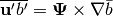 ). Buoyancy
is the negative density anomaly rescaled to have units of acceleration
). Buoyancy
is the negative density anomaly rescaled to have units of acceleration
 , as appropriate for a Boussinesq
fluid. Overlines are used to represent the fields in a coarse-resolution
model, that is, one not resolving the submesoscale eddies. The MLE
fluxes are assumed to occur in addition to resolved or otherwise
parameterized fluxes.
, as appropriate for a Boussinesq
fluid. Overlines are used to represent the fields in a coarse-resolution
model, that is, one not resolving the submesoscale eddies. The MLE
fluxes are assumed to occur in addition to resolved or otherwise
parameterized fluxes.
The FFH parameterization is given by
(187)¶![\begin{aligned}
&{\bf \Psi}_0=C_e \frac{H^2 \nabla {\overline b}^z\times{\hat{\bf z}}}{|f|}\mu(z),&\\
&\!\!\!\!\!\!\mu(z)=\max\left\{0,\left[1-\left(\frac{2 z}{H}+1\right)^2\right]\!\!\!\left[1+\frac{5}{21}\left(\frac{2 z}{H}+1\right)^2\right]\right\},&\nonumber\end{aligned}](../_images/math/bfe5c25d0e5076e423c5c3ec337e75cd9ed9c2c6.png)
where  is mixed layer depth, is the Coriolis
parameter, and
is mixed layer depth, is the Coriolis
parameter, and  is the unit vertical vector. The
overline with subscript on
is the unit vertical vector. The
overline with subscript on  is
understood to be the depth-average of
is
understood to be the depth-average of  over the
mixed layer. The efficiency coefficient
over the
mixed layer. The efficiency coefficient  is approximately
 (Fox-Kemper, Ferrari, and Hallberg 2008). Note that the
parameterization is only nonzero within the mixed layer.
(Fox-Kemper, Ferrari, and Hallberg 2008). Note that the
parameterization is only nonzero within the mixed layer.
An adaptation to (187) that is suitable and justified in a global coarse-resolution model (Fox-Kemper et al. 2010) is:
(188)
 is an appropriate local gridscale of the coarse model,
 is an estimate of the typical local width of mixed layer
fronts, and is a timescale for mixing momentum vertically
across the mixed layer (
is an estimate of the typical local width of mixed layer
fronts, and is a timescale for mixing momentum vertically
across the mixed layer ( 1-10 days). Hosegood, Gregg,
and Alford (2006) suggest is close to the mixed layer
deformation radius
1-10 days). Hosegood, Gregg,
and Alford (2006) suggest is close to the mixed layer
deformation radius  , where is the buoyancy
frequency of the mixed layer stratification. For stability, a lower
cutoff is used:
, where is the buoyancy
frequency of the mixed layer stratification. For stability, a lower
cutoff is used:  where
where
 is chosen in the 1 to 5km range. Likewise, if
is very large, an upper limit near
is chosen in the 1 to 5km range. Likewise, if
is very large, an upper limit near  should be imposed. See Fox-Kemper et al. (2010) for details.
8.1.4.1. Details of Implementation
Coarse Resolution Rescaling: The FFH parameterization
(187) depends on the horizontal density gradient. Coarser
models have weaker gradients than finer, and sparser observations have
weaker gradients than denser. The  factor in
(188) accounts for the expected dependence of horizontal
density gradients on resolution. The vertical buoyancy flux given by
(187) scales as
factor in
(188) accounts for the expected dependence of horizontal
density gradients on resolution. The vertical buoyancy flux given by
(187) scales as
One would like the same vertical buoyancy flux regardless of model
resolution, and the factor is a good approximation
(Fox-Kemper et al. 2010). Note that the horizontal fluxes are not
necessarily accurately rescaled by this method, and the overturning
streamfunction may become very large. However, these submesoscale eddies
are so small that they generally have negligible horizontal fluxes, and
the mixed layer vertical stratification so weak that the parameterized
horizontal fluxes are small even when the streamfunction is large. These
spurious effects are consequences of the resolution rescaling that
should be inconsequential, although the user should keep their spurious
nature in mind.
Timestep Limitation: The overturning streamfunction is thus rescaled
as . The eddy-induced velocity will go as
 , so the timestep is limited as
though the gridscale were instead of . In
practice
, so the timestep is limited as
though the gridscale were instead of . In
practice  is usually smaller than other velocities in the
model–consistent with the small MLE horizontal fluxes. However, it is
possible for the FFH parameterization to require somewhat smaller
timesteps in certain conditions on certain grids, especially with fine
vertical resolution where
is usually smaller than other velocities in the
model–consistent with the small MLE horizontal fluxes. However, it is
possible for the FFH parameterization to require somewhat smaller
timesteps in certain conditions on certain grids, especially with fine
vertical resolution where  may determine the timestep.
Steps are taken in POP to ameliorate this timestep limitation for small
. 1) A minimum value of , , is
used (usually in the one to five km range). 2)
![\min[\Delta s, 1^\circ]/\max[L_f,L_{f,min}]](../_images/math/0f29af25c014d11fcd3ff2d2ab0580bcee6dc22d.png) constrains the
scaleup in very coarse resolution models. As one might expect, the high
latitudes where
constrains the
scaleup in very coarse resolution models. As one might expect, the high
latitudes where  is large are more strongly affected by the
choice of cutoff. The mixed layer frontal scale is often obseved to be
smaller than 5km. However, the buoyancy frequency, , in the
mixed layer is highly sensitive to other parameterization choices (e.g.
maximum diffusivity of mixing in KPP), thus this cutoff is required and
should be adjusted along with other model parameters. Generally, the
cutoff value should be as small as can be safely integrated. In test
cases, a 1km cutoff in POP allows a ML depth nearly 20% shallower in
high latitudes than a 5km cutoff.
is large are more strongly affected by the
choice of cutoff. The mixed layer frontal scale is often obseved to be
smaller than 5km. However, the buoyancy frequency, , in the
mixed layer is highly sensitive to other parameterization choices (e.g.
maximum diffusivity of mixing in KPP), thus this cutoff is required and
should be adjusted along with other model parameters. Generally, the
cutoff value should be as small as can be safely integrated. In test
cases, a 1km cutoff in POP allows a ML depth nearly 20% shallower in
high latitudes than a 5km cutoff.
High-Resolution Usage: The scaling automatically
handles regional variations of eddy scales in a high-resolution model.
If is resolved in some regions – e.g. where the mixed layer
is particularly deep after deep convection – and not in other regions,
the scaling adjusts. A just-resolved front (where  )
has no scale-up and insufficient resolution to form any MLEs. A resolved
front with MLEs permitted but not resolved (
)
has no scale-up and insufficient resolution to form any MLEs. A resolved
front with MLEs permitted but not resolved ( ) is
boosted by the parameterization, and a well resolved feature
(
) is
boosted by the parameterization, and a well resolved feature
( ) has negligible effects from the
parameterization.
) has negligible effects from the
parameterization.
Tracers Other than Buoyancy: The rescaling relies on
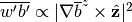 , which is appropriate for the scaling of density
fronts of the near-surface ocean (???). The FFH parameterization is
also used for other tracers, and these fronts will lend similar scaling
behavior to those tracers as well. Thus, the rescaling remains
appropriate.
, which is appropriate for the scaling of density
fronts of the near-surface ocean (???). The FFH parameterization is
also used for other tracers, and these fronts will lend similar scaling
behavior to those tracers as well. Thus, the rescaling remains
appropriate.
Equatorial Regularization: The division by in the scaling
for (187) for  means that this form
cannot be used at the equator. Physically, Boccaletti, Ferrari, and
Fox-Kemper (2007) and Fox-Kemper, Ferrari, and Hallberg (2008) note that
MLEs are largely geostrophic and thus do not restratify in the same way
as the equator is approached. Under typical midlatitude situations, the
growth of instabilities rivals the timescales of mixing events and the
eddy fluxes are only intermittently interrupted. However, as
grows near the equator, frictional constraints
enter. The FFH parameterization (187) is therefore adapted
in (188) to converge to a friction slumping rate (Ferrari and
Young 1997) as the equator is approached. The frictional time constant
should be on the order of the timescale between mixing
events driven by atmospheric synoptic variability–a few days to a few
weeks.
means that this form
cannot be used at the equator. Physically, Boccaletti, Ferrari, and
Fox-Kemper (2007) and Fox-Kemper, Ferrari, and Hallberg (2008) note that
MLEs are largely geostrophic and thus do not restratify in the same way
as the equator is approached. Under typical midlatitude situations, the
growth of instabilities rivals the timescales of mixing events and the
eddy fluxes are only intermittently interrupted. However, as
grows near the equator, frictional constraints
enter. The FFH parameterization (187) is therefore adapted
in (188) to converge to a friction slumping rate (Ferrari and
Young 1997) as the equator is approached. The frictional time constant
should be on the order of the timescale between mixing
events driven by atmospheric synoptic variability–a few days to a few
weeks.
Adjustable Parameters: The scaling (187) has the
simulation-based parameter  . This constant is an
efficiency factor of mixed layer eddies that is apparently constant
across different simulations and should not be changed. However, the
parameters and are not presently known from
observations, theory, or simulations, and therefore they may be tuned to
reduce model bias.
. This constant is an
efficiency factor of mixed layer eddies that is apparently constant
across different simulations and should not be changed. However, the
parameters and are not presently known from
observations, theory, or simulations, and therefore they may be tuned to
reduce model bias.
Discretization: The discretization of advection by the FFH
parameterization is treated identically to that of the advection by the
Gent and McWilliams (1990) parameterization. However, since there is no
division by in the FFH parameterization
(187), eq:parammod, tapering and slope-limiting are not
required.
Regions of Impact: The MLE parameterization is proportional to mixed
layer depth squared and horizontal buoyancy gradient. Thus, regions
where these parameters are large (e.g., western boundary currents, deep
convection sites) will have large effects from the FFH parameterization.
However, the parameterization is not intended to be turned off
regionally, so it may be active in other regions as well. For example,
regions with shallow mixed layers often have weak mixing and weak
convection and thus weak vertical tracer transport, so
 from the FFH parameterization may be
comparable to these processes.
from the FFH parameterization may be
comparable to these processes.
8.2. Horizontal Viscosity
8.2.1. Laplacian Horizontal Viscosity
The spatial discretization of the standard Laplacian horizontal friction
terms with a spatially varying viscosity  given by
(29) is described in Sec. Horizontal Friction.
given by
(29) is described in Sec. Horizontal Friction.
8.2.2. Biharmonic Horizontal Viscosity
In analogy to the biharmonic diffusion operator (153), the biharmonic viscosity is constructed by applying the Laplacian-like operator (28) twice. Specifically,
(189)
with a similar expression for  . The
superscripts (4) and (2) refer to biharmonic and harmonic operators, and
. The
superscripts (4) and (2) refer to biharmonic and harmonic operators, and
 is given by (28) with
 .
.  is the biharmonic viscosity, which may
be spatially varying, and should be negative for positive-definite
dissipation of kinetic energy. Here the biharmonic viscosity is
sandwiched between the two applications of the harmonic operator. An
alternate approach (not implemented in the code) is to include the
square-root of
is the biharmonic viscosity, which may
be spatially varying, and should be negative for positive-definite
dissipation of kinetic energy. Here the biharmonic viscosity is
sandwiched between the two applications of the harmonic operator. An
alternate approach (not implemented in the code) is to include the
square-root of  inside the second derivative of each
harmonic operator (Griffies and Hallberg 2000).
inside the second derivative of each
harmonic operator (Griffies and Hallberg 2000).
8.2.3. Anisotropic Horizontal Viscosity
An anisotropic formulation of the friction terms in the momentum
equation was first introduced into an ocean GCM by Large et al. (2001).
This was implemented in a model with a spherical polar grid, and their
formulation was specifically tied to that coordinate system. A more
general formulation of anisotropic viscosity that can be applied in any
general orthogonal coordinate system was developed by Smith and
McWilliams (2003) ((2003), hereafter SM), and is implemented in the POP
code. The friction operator is formulated as the divergence of a viscous
stress tensor which is linearly related to the velocity gradients. The
general anisotropic formulation of the stress involves four independent
viscous coefficients, as well as a unit vector  that
specifies a preferred horizontal direction which breaks the transverse
isotropy. The coefficients and the direction vector may vary in both
space and time. A modification of the original formulation has been
implemented by Jochum et al. (2008) that changes the values, but not the
structure of viscosity. Equations (195) and (197) are modified
from the SM version to allow for a better representation of equatorial
and high latitude boundary currents.
that
specifies a preferred horizontal direction which breaks the transverse
isotropy. The coefficients and the direction vector may vary in both
space and time. A modification of the original formulation has been
implemented by Jochum et al. (2008) that changes the values, but not the
structure of viscosity. Equations (195) and (197) are modified
from the SM version to allow for a better representation of equatorial
and high latitude boundary currents.
SM discuss two different reduced forms involving only two viscous
coefficients, and  . In both of these forms, the
friction operator in Cartesian coordinates has the following approximate
form if the -coordinate is aligned with :
. In both of these forms, the
friction operator in Cartesian coordinates has the following approximate
form if the -coordinate is aligned with :
(190)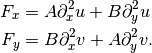
Thus, the friction acts to diffuse momentum along the direction
with viscosity , and perpendicular to
with viscosity ; this is true for the
general operator, even when the coordinates are not aligned with
.
The three independent elements  ,
,  and
and  of the symmetric transverse stress tensor
 are linearly related to the elements of the
rate-of-strain tensor
are linearly related to the elements of the
rate-of-strain tensor  (where the subscripts 1 and 2
refer to the and coordinates, respectively). In the
first form discussed by SM, which is currently implemented in the code,
the stress and strain-rate are related by
(where the subscripts 1 and 2
refer to the and coordinates, respectively). In the
first form discussed by SM, which is currently implemented in the code,
the stress and strain-rate are related by
(191)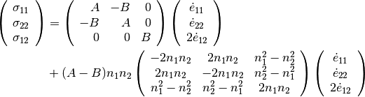
where  and
and  are the components of
along the and coordinates,
respectively. In the second two-coefficient form, the relation between
the stress and strain-rate is also given by (191), except
that the first matrix inside the brackets on the right is replaced by
are the components of
along the and coordinates,
respectively. In the second two-coefficient form, the relation between
the stress and strain-rate is also given by (191), except
that the first matrix inside the brackets on the right is replaced by
The second form is actually independent of the horizontal divergence, and can be written in the more compact form:
(192)¶![\begin{aligned}
\left( \begin{array}{c}
\sigma_{_T} \\
\sigma_{_S} \end{array}\right)
=
\Biggl[
& \left( \begin{array}{cc}
A+B & 0 \\
0 & 2B \end{array} \right) \\
& + 2(A-B)n_{1}n_{2}
\left( \begin{array}{cc}
-2n_1 n_2 & n_1^2 - n_2^2 \\
n_1^2 - n_2^2 & 2n_1 n_2 \end{array} \right)
\Biggr]
\left( \begin{array}{c}
\dot{e}_{_T} \\
\dot{e}_{_S} \end{array}\right). \nonumber \end{aligned}](../_images/math/927e102aec10d9638dae5145127aa4df435f6a26.png)
where  ,
,
 ,
,
 and
and
 . The two forms are equivalent up to
terms proportional to the horizontal velocity divergence
. The two forms are equivalent up to
terms proportional to the horizontal velocity divergence
 which is very
small compared to typical velocity gradients in geophysical flows, as
discussed by SM. The first form was essentially constructed so that it
exactly produces the Cartesian friction operator (190),
whereas the second form was derived as the limit
which is very
small compared to typical velocity gradients in geophysical flows, as
discussed by SM. The first form was essentially constructed so that it
exactly produces the Cartesian friction operator (190),
whereas the second form was derived as the limit
 of the general four-coefficient
form of the stress. For this reason, the second form has a more sound
physical basis, however, the results using the two forms should in most
cases be very similar.
of the general four-coefficient
form of the stress. For this reason, the second form has a more sound
physical basis, however, the results using the two forms should in most
cases be very similar.
In both forms the stress is invariant under a rotation of
by  . Currently there are three
options in the code for the field of unit vectors :
(1) aligned along the flow direction
(
. Currently there are three
options in the code for the field of unit vectors :
(1) aligned along the flow direction
( ); (2) aligned with due east
(or, equivalently, with any of the four cardinal directions); and (3)
aligned with the local grid coordinates (in polar coordinates this is
equivalent to (2), but it is different in general orthogonal coordinate
systems such as the displaced-pole grids described in Sec. Global Orthogonal Grids).
With any of these choices, the isotropic limit is obtained by equating
the two coefficients
); (2) aligned with due east
(or, equivalently, with any of the four cardinal directions); and (3)
aligned with the local grid coordinates (in polar coordinates this is
equivalent to (2), but it is different in general orthogonal coordinate
systems such as the displaced-pole grids described in Sec. Global Orthogonal Grids).
With any of these choices, the isotropic limit is obtained by equating
the two coefficients  . The first form reduces to the original
anisotropic formulation of Large et al. (2001) when
is oriented eastward.
. The first form reduces to the original
anisotropic formulation of Large et al. (2001) when
is oriented eastward.
The spatial discretization of the anisotropic friction operator is described in detail by SM, and will only be briefly reviewed here. The basic idea of this approach is to take advantage of the fact that the friction operator can be written as the functional derivative of the area-integrated energy dissipation rate. Using the no-slip lateral boundary conditions on the velocity, it can be shown that the domain-averaged dissipation of kinetic energy due to friction is given by
where is the friction vector and  is the
energy dissipation rate:
is the
energy dissipation rate:

To ensure positive-definite dissipation of kinetic energy, the viscous
coefficients must be chosen to satisfy  . It can be
shown that in the first form this leads to the constraint
. It can be
shown that in the first form this leads to the constraint
 , whereas the second form has the less restrictive
constraint
, whereas the second form has the less restrictive
constraint  . The
. The  component of the friction is given by
where  denotes a functional derivative
with respect to the component of the velocity.
The procedure for deriving the discrete operator is to first discretize
the functional, making sure that the discrete form is positive definite,
and then take its derivatives with respect to the velocity components at
a given point on the computational grid; this yields a friction operator
at that point that is guaranteed to dissipate kinetic energy. As was
done in the case of the GM operator described in Sec. The Gent-McWilliams Parameterization, the
method of discretizing the functional is to subdivide each horizontal
cell into four subcells (see Figure7.1. , with the central
point interpreted as a U-point). This allows all quantities (such as
viscous coefficients, gradients of velocities, etc.) required to
construct the dissipation rate to be assigned a unique value in each
subcell. In this manner the components of the strain-rate tensor are
computed in each subcell, and from these the stresses are computed using
(191). The specific details of the derivation are given
by SM, and we will only quote the final result here. The discrete
friction operator has the form
denotes a functional derivative
with respect to the component of the velocity.
The procedure for deriving the discrete operator is to first discretize
the functional, making sure that the discrete form is positive definite,
and then take its derivatives with respect to the velocity components at
a given point on the computational grid; this yields a friction operator
at that point that is guaranteed to dissipate kinetic energy. As was
done in the case of the GM operator described in Sec. The Gent-McWilliams Parameterization, the
method of discretizing the functional is to subdivide each horizontal
cell into four subcells (see Figure7.1. , with the central
point interpreted as a U-point). This allows all quantities (such as
viscous coefficients, gradients of velocities, etc.) required to
construct the dissipation rate to be assigned a unique value in each
subcell. In this manner the components of the strain-rate tensor are
computed in each subcell, and from these the stresses are computed using
(191). The specific details of the derivation are given
by SM, and we will only quote the final result here. The discrete
friction operator has the form
(193)¶![\begin{aligned}
F_x = &\frac{1}{V}[
\overline{h_2\sigma_{11}}^e - \overline{h_2\sigma_{11}}^w
+ \overline{h_1\sigma_{12}}^n - \overline{h_1\sigma_{12}}^s \nonumber \\
&+\frac{1}{2}\,(h_2^n k_2^n \overline{h_1\sigma_{12}}^n
+h_2^s k_2^s \overline{h_1\sigma_{12}}^s) \nonumber \\
&-\frac{1}{2}\,(h_1^e k_1^e \overline{h_2\sigma_{22}}^e
+h_1^w k_1^w \overline{h_2\sigma_{22}}^w)]
\nonumber \\
\nonumber \\
F_y = &\frac{1}{V}[
\overline{h_1\sigma_{22}}^n - \overline{h_1\sigma_{22}}^s
+ \overline{h_2\sigma_{12}}^e - \overline{h_2\sigma_{12}}^w \nonumber \\
&+\frac{1}{2}\,(h_1^e k_1^e \overline{h_2\sigma_{12}}^e
+h_1^w k_1^w \overline{h_2\sigma_{12}}^w) \nonumber \\
&-\frac{1}{2}\,(h_2^n k_2^n \overline{h_1\sigma_{11}}^n
+h_2^s k_2^s \overline{h_1\sigma_{11}}^s)]
\end{aligned}](../_images/math/b93cb7577d3a46324496e40ee57355070a683f8d.png)
where  and
and  are the components of the friction
operator along the two general orthogonal coordinate directions
and . The factors and
are the components of the friction
operator along the two general orthogonal coordinate directions
and . The factors and  are
distances between grid points along the two coordinate directions, and
are
distances between grid points along the two coordinate directions, and
 and
and  are metric factors proportional to the
derivatives of and in the and
directions, respectively. The overbars denote an average over
the four subcells surrounding a given face (denoted by the superscript
,
are metric factors proportional to the
derivatives of and in the and
directions, respectively. The overbars denote an average over
the four subcells surrounding a given face (denoted by the superscript
,  , , or , for the north, south,
east and west faces), and
, , or , for the north, south,
east and west faces), and  is the full cell area. For a more
detailed description of the quantities in (193), see the
appendix of SM.
is the full cell area. For a more
detailed description of the quantities in (193), see the
appendix of SM.
The viscous coefficients are assumed to have a constant value within a
given full cell, i,e., all four subcells within each full cell have the
same values of the coefficients and . There are
currently three options in the code for the form of the viscous
coefficients: (1) constant values of and in both
space and time, (2) spatially varying but constant in time; and (3)
Smagorinsky-type nonlinear coefficients that depend on the local
deformation rate and hence vary in both space and time. In options (2)
and (3), the viscosities are tapered if they exceed one-half the viscous
CFL limit. Specifically, both and are tapered as
follows:
(194)
where  is the model momentum timestep, and
  and
and
 are the grid spacings in the two coordinate directions. For
option (1), and are simply set to different,
constant values. The model does not enforce the limit, if they exceed
are the grid spacings in the two coordinate directions. For
option (1), and are simply set to different,
constant values. The model does not enforce the limit, if they exceed
 ; only a warning message is printed. If
 , the integration is terminated with an error exit.
The spatial dependence of the coefficients is computed following Jochum
et al. (2008), which also demonstrates their importance for climate. The
two primary design criteria are to have viscosity at values appropriate
for the parameterization of missing meso-scale eddies wherever possible
and to use other values only where required by the numerics. The
parallel coefficient  is given by
(195)
The first part represents a numerical, Munk viscous western boundary constraint with
(196)
where causes to fall off as fast as possible
away from the western boundaries. Here,  is the zonal
coordinate of the
is the zonal
coordinate of the  grid point east of the nearest western
boundary and
grid point east of the nearest western
boundary and  is a length scale. Viscosity is not similarly
increased near zonal and eastern boundaries because doing so does not
reduce numerical noise. Also,
is a length scale. Viscosity is not similarly
increased near zonal and eastern boundaries because doing so does not
reduce numerical noise. Also,  is a
dimensionless coefficient, and is the meridional gradient
of the Coriolis parameter.
is a
dimensionless coefficient, and is the meridional gradient
of the Coriolis parameter.  is a physical, lower bound
set to account for all the missing mesoscale eddy activity. The
perpendicular coefficient
is a physical, lower bound
set to account for all the missing mesoscale eddy activity. The
perpendicular coefficient  is constructed as
(197)¶![B_1 = \max {\biggl \{} c_3\ \beta \ dx^3 \ exp(-p(x)^2),\ B_{eddy}
\ {\bigl (} 1 + c_2 (1 - cos [2\phi^\prime] ) {\bigr )} {\biggr \}}.](../_images/math/3775b3fae736683a1777e26fc5b9a5ebbb1ef4a1.png)
The first part represents again the Munk viscous western boundary
constraint. In the second part,  and
and
 represents a physical lower bound. This form allows
to be small at the equator and increase poleward for
latitude between
represents a physical lower bound. This form allows
to be small at the equator and increase poleward for
latitude between  , using the dimensionless coefficient
 . A preferred option is to set
 , so that becomes
equal to poleward of
, so that becomes
equal to poleward of  . In most applications,
however, is set equal to .
. In most applications,
however, is set equal to .
To obtain the final distributions of and , the
viscosities are tapered if they exceed half of the viscous CFL limit:
(198)
8.2.3.1. Smagorinsky Nonlinear Viscous Coefficients
Jochum et al. (2008) shows that Smagorinsky-type nonlinear viscosity
leads to excessive viscosity along boundaries and the equator. However,
the code is still set up to optionally allow for Smagorinksy-type
nonlinear dependence of the coefficients on the deformation rate
(Smagorinsky 1993) if the anisotropic functional discretization
described in Sec. Anisotropic Horizontal Viscosity is used. This option is not available
with the simple Laplacian-like friction operator given by
(29). An isotropic form with the same Smagorinsky-type
nonlinear viscosity can be obtained by simply setting the two
anisotropic viscous coefficients and equal to one
another.
The deformation rate  is proportional to the norm of the
strain-rate tensor:
is proportional to the norm of the
strain-rate tensor:
(199)
This is particularly easy to evaluate because the strain-rate tensor is
already computed in the code. Specifically, the nonlinear coefficients
and are given by
(200)¶![\begin{aligned}
A &= \min\left[\max\left(C_{_{A}} \dot{D}\,
ds^2,V_{_{A}}\,ds\right),\: \frac{1}{2}A_{\mathrm{cfl}}\right]
\nonumber \\
B &= \min\left[\max\left(C_{_{B}} \dot{D}\,
ds^2,V_{_{B}}\,ds\right),\:\frac{1}{2}A_{\mathrm{cfl}}\right]
\end{aligned}](../_images/math/8af8ea67adcfa7af483be1aaf36a5c9bfc35a467.png)
where  is the minimum grid spacing in the
two coordinate directions.
is the minimum grid spacing in the
two coordinate directions.  and
and  are
dimensionless coefficients of order 1, and
are
dimensionless coefficients of order 1, and  and
and
 are velocity scales associated with the grid Reynolds
number which determine a minimum background viscosity in regions where
the nonlinear viscosity is too small to control grid-point noise.
Typically and are order 1
cm s. is the maximum viscosity
allowed by the viscous CFL limit, see (194). The advantage
of the nonlinear viscosities (200) is that they selectively
apply the friction operator in regions of strong shear.
are velocity scales associated with the grid Reynolds
number which determine a minimum background viscosity in regions where
the nonlinear viscosity is too small to control grid-point noise.
Typically and are order 1
cm s. is the maximum viscosity
allowed by the viscous CFL limit, see (194). The advantage
of the nonlinear viscosities (200) is that they selectively
apply the friction operator in regions of strong shear.
In moderate resolution configurations of POP, the Smagorinsky coefficients have been modified in a similar manner to the anisotropic coefficients in Large et al. (2001) described above. Again the reason is to control numerical noise in the solutions. Equation (200) has been modified such that
(201)¶![\begin{aligned}
A &= \min \left[ \max \left( C_A F_A(\phi)\dot{D}ds^2, A_1 \right),
\ \frac{1}{2} A_\mathrm{cfl} \right], \nonumber \\
B &= \min \left[ \max \left( C_B F_B(\phi)\dot{D}ds^2, B_1 \right),
\ \frac{1}{2} A_\mathrm{cfl} \right],
\end{aligned}](../_images/math/2510e5eeb14340fc42b44da9a96fef9fa022d5b2.png)
with
(202)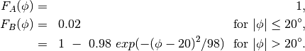
Here,  is the minimum grid spacing in
the two coordinate directions.
is the minimum grid spacing in
the two coordinate directions.  and
and  are
dimensionless coefficients of order 1 whose latitudinal dependencies are
given by
are
dimensionless coefficients of order 1 whose latitudinal dependencies are
given by  and
and  , respectively. The
positive-definite dissipation of kinetic energy is enforced by the last
equation in (198). Where these nonlinear viscosities are too small,
and , with the same formulations as in the
previous section, provide lower limits to control any grid-point noise.
, respectively. The
positive-definite dissipation of kinetic energy is enforced by the last
equation in (198). Where these nonlinear viscosities are too small,
and , with the same formulations as in the
previous section, provide lower limits to control any grid-point noise.
8.3. Vertical Mixing
Vertical mixing is treated using the spatial discretizations presented
in sections Vertical Tracer Diffusion and Vertical Friction. The implicit
time discretizations are presented in Secs. Implicit Vertical Diffusion,
Tridiagonal Solver, and Semi-Implicit Treatment of Coriolis and Vertical Friction Terms. POP contains three
different parameterizations for computing the vertical diffusivity
(VDC in the code) and viscosity (VVC in the
code): constant coefficients, a parameterization based on the gradient
Richardson number by Pacanowski and Philander (1981) and the K-profile
parameterization (KPP) of (???).
8.3.1. Convection
Convective instability can be handled in two ways within the code. If implicit vertical mixing is used, convection is generally treated by assigning a very large diffusivity and viscosity when the density profile between two cells in the vertical direction is statically unstable. The diffusivity and viscosity in each case is determined at run time through namelist inputs.
If explicit vertical mixing is used, convection is usually treated using
convective adjustment. During convective adjustment, multiple passes
through the water column are performed to check for stability and to
adjust tracer values. Each pass in turn consists of two sweeps. The
first sweep checks odd-valued vertical levels; the second checks
even-valued levels. At each level , the stability between level
and level  is checked (see below for stability
criterion). If the two cells are found to be unstably-stratified, the
tracer in each level is adjusted using
is checked (see below for stability
criterion). If the two cells are found to be unstably-stratified, the
tracer in each level is adjusted using
(203)
If tracer acceleration is being used, the thicknesses  are
adjusted by the acceleration factor
are
adjusted by the acceleration factor
(204)
Instability can be determined using one of two methods. In both the Richardson number parameterization and KPP, the Richardson number is computed and the column is unstable when the Richardson number is less than zero. The calculation of Richardson number differs slightly between the two and is shown in each section below.
If the Richardson number is not computed, stability is determined by
adiabatically displacing a water mass from the current vertical level
to the level just below. The density of the parcel
after this displacement, denoted  , is computed by
calling the equation of state with the temperature and salinity from
level , but evaluating the equation of state at level
. If the density after the displacement is greater than the
actual density at the level , the column is unstable.
, is computed by
calling the equation of state with the temperature and salinity from
level , but evaluating the equation of state at level
. If the density after the displacement is greater than the
actual density at the level , the column is unstable.
8.3.2. Constant Vertical Viscosity
If this option is chosen, the vertical diffusivity VDC and vertical viscosity VVC are simply constant at all levels and for all tracers. The scalar constant values are determined at run time through namelist input.
8.3.3. Richardson Number Dependent Mixing
In this parameterization, the vertical diffusivity and viscosity are functions of the Richardson number,
(205)
where the velocities are evaluated at tracer points and
is simply a small number to avoid dividing by zero.
The particular functional forms for the diffusivity (VDC)
and viscosity (VVC) used in the code are
(206)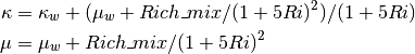
where the background values  and
and  and
Richardson mixing coefficient
and
Richardson mixing coefficient  are determined at run
time through namelist input. Note that the Richardson number used for
the viscosity has been averaged from tracer points to
velocity points.
are determined at run
time through namelist input. Note that the Richardson number used for
the viscosity has been averaged from tracer points to
velocity points.
8.3.4. The KPP Boundary-Layer Parameterization
The full KPP parameterization is detailed in (???), hereafter LMD,
so only a general overview plus specifics of the current POP
implementation and later modifications (see also Appendix A of
Danabasoglu et al. (2006)) are described here. The scheme provides all
the coefficients required to compute the vertical mixing contributions
to both  in (7), and
 in (11). As such, it
should not be used in conjunction with any other parameterization of
vertical mixing. Implicit vertical mixing is required to solve
(7) and a modified version of (13);
namely,
in (11). As such, it
should not be used in conjunction with any other parameterization of
vertical mixing. Implicit vertical mixing is required to solve
(7) and a modified version of (13);
namely,
(207)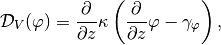
where the additional non-local transport term,  is non-zero only in convective (unstable) forcing, and above a diagnosed
boundary layer depth, . In the ocean interior below ,
the viscosity,
is non-zero only in convective (unstable) forcing, and above a diagnosed
boundary layer depth, . In the ocean interior below ,
the viscosity,  , and diffusivity,
  ,
represent very different physics than their boundary layer,
,
represent very different physics than their boundary layer,
 , counterparts, denoted
  and
and
 , respectively.
The inputs to the scheme on the tracer grid are the surface forcing and
vertical profiles of temperature and salinity. The specific forcings are
the surface friction velocity,  , both the solar,
 , and non-solar,
  , buoyancy fluxes, and the
kinematic surface tracer fluxes,
, buoyancy fluxes, and the
kinematic surface tracer fluxes,  . From
the equation of state and its buoyancy form,
. From
the equation of state and its buoyancy form,  ,
derived profiles are the thermal and haline Boussinesq coefficients,
,
derived profiles are the thermal and haline Boussinesq coefficients,
 and
and  , the local buoyancy difference at
each interface,
, the local buoyancy difference at
each interface,  , and the excess buoyancy of
first level water when moved down to each grid level,
, and the excess buoyancy of
first level water when moved down to each grid level,
(208)
The local vertical shear at each interface is squared before being
averaged onto the tracer grid, as  . In contrast, the
square of velocity differences with the first level on the tracer grid
are taken as the maximum from the four neighboring velocity points:
. In contrast, the
square of velocity differences with the first level on the tracer grid
are taken as the maximum from the four neighboring velocity points:
(209)
For vertical resolutions of  or less, excessive sensitivity
can be avoided if
or less, excessive sensitivity
can be avoided if  and
and  in the
above equations are replaced by averages over the upper 10% of the
boundary layer (LMD). A local gradient Richardson number,
in the
above equations are replaced by averages over the upper 10% of the
boundary layer (LMD). A local gradient Richardson number,  ,
buoyancy frequency, , and density ratio,
,
buoyancy frequency, , and density ratio,  , on
the tracer grid are computed as
, on
the tracer grid are computed as
(210)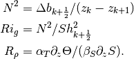
It is then a five step process to complete the algorithm, as described below. First, the interior mixing coefficients are computed at all model interfaces, on the tracer grid, as if there were no boundary layer scheme. These are the sum of individual viscosities and diffusivities corresponding to a number (currently up to four) of different physical processes:
(211)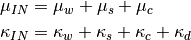
The first coefficients on the right hand side are background values.
With the exception of the surface mixed layer and the bottom boundary
layer, the parameterizations of which are documented below, the ocean is
mostly adiabatic. However, even there diapycnal mixing happens due to
internal waves and other mechanisms. In POP this is represented by the
background diffusivity and the background viscosity
. Their vertical variation has the general form
(212)
where  equals the vertical diffusivity at
  ,
,
 is the amplitude of variation,
  is the inverse
length scale of the transition region, and
is the inverse
length scale of the transition region, and  is the depth
where diffusivity equals . The form allows for an increase
in diffusivity with depth, as a crude parameterization of the observed
increase in deep mixing over rough topography.
is the depth
where diffusivity equals . The form allows for an increase
in diffusivity with depth, as a crude parameterization of the observed
increase in deep mixing over rough topography.  is only
poorly constrained by observations and thus set to a constant value of
10. , too, used to be only weakly constrained by
observations, but since the release of CCSM3 in 2004 it became clear
that there is not only a latitudinal structure to , but
also that variations to it can have a dramatic impact on climate (Jochum
and Potemra 2008). Thus, the value of has been changed
from constant values of typically
is only
poorly constrained by observations and thus set to a constant value of
10. , too, used to be only weakly constrained by
observations, but since the release of CCSM3 in 2004 it became clear
that there is not only a latitudinal structure to , but
also that variations to it can have a dramatic impact on climate (Jochum
and Potemra 2008). Thus, the value of has been changed
from constant values of typically  to 0.17
 (bckgrnd_vdc1 + bckgrnd_vdc_eq = 0.16 + 0.01 = 0.17)
mostly everywhere. The regions with different values are the Banda Sea
(bckgrnd_vdc_ban = 1.0 ), the latitude bands around
30
(bckgrnd_vdc1 + bckgrnd_vdc_eq = 0.16 + 0.01 = 0.17)
mostly everywhere. The regions with different values are the Banda Sea
(bckgrnd_vdc_ban = 1.0 ), the latitude bands around
30 N/S (bckgrnd_vdc1 + bckgrnd_vdc_eq +
bckgrnd_vdc_psim = 0.3 ), and the equator
(bckgrnd_vdc_eq = 0.01 ). The theories and observations
that led to this new structure, as well as their impact on climate, are
discussed in Jochum (2009).
N/S (bckgrnd_vdc1 + bckgrnd_vdc_eq +
bckgrnd_vdc_psim = 0.3 ), and the equator
(bckgrnd_vdc_eq = 0.01 ). The theories and observations
that led to this new structure, as well as their impact on climate, are
discussed in Jochum (2009).
The viscosity and diffusivity associated with shear instability mixing
are equal ( ) and parameterized as a function of
:
) and parameterized as a function of
:
(213)¶![\mu_s = \kappa_s = \kappa_s^0 \left[1-
\left(\frac{Ri_g}{Ri_0}\right)^2 \right]^3,
\quad 0 < Ri_g < Ri_0 .](../_images/math/43b2fb6a2b79f67a280ccc795afc7ace8e933d7c.png)
For an unstable profile with negative the coefficients
remain constant at  (rich_mix () in
namelist), and are zero for all
(rich_mix () in
namelist), and are zero for all  . This function
falls most rapidly near
. This function
falls most rapidly near  , where it approximates
the onset of shear instability. In this neighborhood rapid changes in
can cause instabilities to develop in the vertical, but
these are largely controlled by vertically smoothing
profiles. A
, where it approximates
the onset of shear instability. In this neighborhood rapid changes in
can cause instabilities to develop in the vertical, but
these are largely controlled by vertically smoothing
profiles. A  smoother is can be applied repeated a
specified number of times.
smoother is can be applied repeated a
specified number of times.
Convective instability in the interior ocean is relieved by setting the
mixing coefficients,  and
and  , to large values
whenever the density profile is unstable,
, to large values
whenever the density profile is unstable,  . Otherwise, they
are set to zero.
. Otherwise, they
are set to zero.
Second, double diffusion processes have the potential to significantly
enhance diffusivities, with the governing parameter.
Their effects on viscosity are ignored in (211), because they
are not well known and because the large value of ,
relative to in (211) means that they are
unlikely to be dominant. In the salt fingering regime (destabilizing
salinity profile and  ), the
diffusivity is a fit to observational estimates (St.Laurent and Schmitt
1999)
), the
diffusivity is a fit to observational estimates (St.Laurent and Schmitt
1999)
(214)¶![\kappa_d = \kappa_d^0 \left[1-\frac{{R_{\rho}-1}}{{R_{\rho}^0 -1}}\right]^3.](../_images/math/0d05c07b8f52e95d0905b346d3c85ecdfbae220f.png)
The values of  are internally set to
  for salt and
  for heat. Diffusive convective
instability occurs where the temperature is destabilizing and
for heat. Diffusive convective
instability occurs where the temperature is destabilizing and
 . For temperature
(215)¶![\begin{aligned}
\kappa_d = \mathrm{VISCM} \times .909
\exp\left(4.6\exp\left[-.54\left(R_{\rho}^{-1} - 1\right)\right]\right),
\end{aligned}](../_images/math/dc2805542e69ae04f82d932ff08f2a5ecfec8e08.png)
where VISCM is molecular viscosity. Multiplying this diffusivity by a
(216)
gives diffusivities for other tracers, including salt.
Third, the diagnostic boundary layer depth, h, is determined on the tracer grid. A bulk Richardson number relative to the surface is defined at each vertical level as
(217)
LMD gives the rationale and expression for the shear contribution from
unresolved turbulence,  . The buoyancy frequency in this
expression is taken from (210) at the interface below the
boundary layer depth. Furthermore, the factor which accounts for
smoothing of the buoyancy profile at the entrainment depth is an
empirical function of this frequency, and ranges linearly from 2.1 at
zero to 1.7 at
. The buoyancy frequency in this
expression is taken from (210) at the interface below the
boundary layer depth. Furthermore, the factor which accounts for
smoothing of the buoyancy profile at the entrainment depth is an
empirical function of this frequency, and ranges linearly from 2.1 at
zero to 1.7 at  and all higher frequencies. The
boundary layer depth is equated to the shallowest depth where
and all higher frequencies. The
boundary layer depth is equated to the shallowest depth where
 equals an internally specified critical value,
 (LMD), using a quadratic, rather than linear,
interpolation whenever possible. With stabilizing surface forcing,
options exist (namelist flag lcheckekmo = .true.) to limit to
be no greater than either the Ekman depth (
(LMD), using a quadratic, rather than linear,
interpolation whenever possible. With stabilizing surface forcing,
options exist (namelist flag lcheckekmo = .true.) to limit to
be no greater than either the Ekman depth ( ), or the
Monin-Obukhov depth (
), or the
Monin-Obukhov depth ( ), where
 is the von Karman constant, and the surface buoyancy flux,
 , is plus a fraction of (LMD).
The grid level immediately below h is denoted as
, is plus a fraction of (LMD).
The grid level immediately below h is denoted as  .
.
Fourth, the boundary layer mixing coefficients are computed on the
tracer grid and replace the interior values from step 1, for
 . The analytic expression is
(218)
where  varies from 0 to 1 over the boundary
layer. The turbulent velocity scales,
varies from 0 to 1 over the boundary
layer. The turbulent velocity scales,  and
and
 are usually proportional to , but become
proportional to the convective velocity scale as
are usually proportional to , but become
proportional to the convective velocity scale as
 in convective forcing (see LMD for details).
The shape function is a cubic polynomial whose coefficients are chosen
such that
in convective forcing (see LMD for details).
The shape function is a cubic polynomial whose coefficients are chosen
such that  , fluxes vary linearly near the surface, and
interior (excluding the convective contributions) and boundary layer
coefficients, and their first vertical derivatives, are continuous at
, fluxes vary linearly near the surface, and
interior (excluding the convective contributions) and boundary layer
coefficients, and their first vertical derivatives, are continuous at
 . An inherent bias to shallow boundary layers is ameliorated
by making the coefficients at the
. An inherent bias to shallow boundary layers is ameliorated
by making the coefficients at the  interface
linear combinations of the interior values at this interface, and the
boundary layer values at both the interface and at the nearest higher
level,
interface
linear combinations of the interior values at this interface, and the
boundary layer values at both the interface and at the nearest higher
level,  (LMD). This feature is less important when
quadratic interpolation is used to find the boundary layer depth.
(LMD). This feature is less important when
quadratic interpolation is used to find the boundary layer depth.
In convective (unstable) forcing situations the nonlocal term is non-zero, and evaluated as
(219)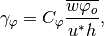
where the constant  is prescribed as in LMD.
Fifth and finally, the viscosity is averaged from the tracer grid to velocity points.
8.3.5. Tidally Driven Mixing
The tidally driven mixing parameterization implemented in CCSM POP is
described in Jayne (2009). There are multiple parameterizations of
mixing phenomena in the model (as well as numerical mixing), however
here we are only concerned with the vertical mixing in the interior away
from the surface boundary layer. The tidally driven vertical mixing
parameterization of Laurent, Simmons, and Jayne (2002) was implemented
in a similar fashion as in Simmons et al. (2004). This mixing is added
to the interior mixing part of the KPP vertical mixing scheme as another
component,  , in equation (211):
(220)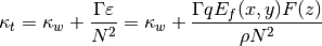
We note that essentially replaces in
equation (211), because is already included in
.
The parameterization for the vertical diffusivity is related to the
turbulent dissipation of internal wave dissipation using the Osborn
(1980) relation and depends on the stratification, . The mixing
efficiency of turbulence is set by  and is taken to be the
canonical value of
and is taken to be the
canonical value of  (Osborn 1980). The tidal
dissipation efficiency is given by the parameter,
(Osborn 1980). The tidal
dissipation efficiency is given by the parameter,
 , and represents the part of the internal wave
energy flux,
, and represents the part of the internal wave
energy flux,  , that is estimated to be dissipated locally
(Laurent and Garrett 2002). The rest of the internal wave energy
, that is estimated to be dissipated locally
(Laurent and Garrett 2002). The rest of the internal wave energy
 is presumed to radiate to the far field and
contribute to the background internal wave field (Garrett and Munk
1975). The vertical structure function,
is presumed to radiate to the far field and
contribute to the background internal wave field (Garrett and Munk
1975). The vertical structure function,  , models the
distribution of the turbulent mixing in the vertical, and is implemented
as a simple exponential decaying upwards away from the bottom, with a
vertical scale of
, models the
distribution of the turbulent mixing in the vertical, and is implemented
as a simple exponential decaying upwards away from the bottom, with a
vertical scale of  m (Laurent and Nash 2004):
(221)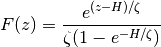
so it is normalized such that vertical integral over the water column is unity (Laurent, Simmons, and Jayne 2002). In the POP code implementation, the vertical exponential function is summed numerically for the normalization.
The constant background value of is an attempt to model
the low level of mixing in the ocean in areas away from topography
(Gregg 1987). Exactly what contributes the mechanical energy required to
maintain order  background
diffusivity is less clear. However, it is the order of magnitude
expected from the self-interaction of the background Garrett-Munk
internal wave spectrum (Gregg 1987; Gregg 1989; Hibiya, Nagasawa, and
Niwa 2006).
background
diffusivity is less clear. However, it is the order of magnitude
expected from the self-interaction of the background Garrett-Munk
internal wave spectrum (Gregg 1987; Gregg 1989; Hibiya, Nagasawa, and
Niwa 2006).
The vertical viscosity is calculated from the vertical diffusivity
assuming  , as is typically done in other
parameterizations (e.g. KPP). In the limit of
, as is typically done in other
parameterizations (e.g. KPP). In the limit of  (or becoming negative), both the vertical diffusivity and viscosity are
capped at
(or becoming negative), both the vertical diffusivity and viscosity are
capped at  . This is a
departure from the original Simmons et al. (2004) who instead impose a
lower limit on of
. This is a
departure from the original Simmons et al. (2004) who instead impose a
lower limit on of  (additionally convective mixing was used to limit negative
stratification regions). In addition, both the diffusivity and viscosity
coefficients within the two bottom-most grid cells are checked and
modified, if necessary, to ensure that they do not diminish with depth
near the bottom topography. Such decreasing-with-depth diffusivities
result from large in a few isolated grid points, likely due
to advection errors. Modifications of these diffusivity coefficients,
e.g., capping the diffusivities, change the energy consistency of the
scheme, and so should be chosen carefully. One other change from the
original Simmons et al. (2004) implementation was that the
parameterization was applied everywhere, whereas they arbitrarily
limited it to depths greater than 1000m. The conversion of tidal energy
into internal waves that occurs in the deep ocean also occurs along the
shelf break, so there is no reason to limit it to the abyssal ocean.
(additionally convective mixing was used to limit negative
stratification regions). In addition, both the diffusivity and viscosity
coefficients within the two bottom-most grid cells are checked and
modified, if necessary, to ensure that they do not diminish with depth
near the bottom topography. Such decreasing-with-depth diffusivities
result from large in a few isolated grid points, likely due
to advection errors. Modifications of these diffusivity coefficients,
e.g., capping the diffusivities, change the energy consistency of the
scheme, and so should be chosen carefully. One other change from the
original Simmons et al. (2004) implementation was that the
parameterization was applied everywhere, whereas they arbitrarily
limited it to depths greater than 1000m. The conversion of tidal energy
into internal waves that occurs in the deep ocean also occurs along the
shelf break, so there is no reason to limit it to the abyssal ocean.
The internal wave energy map, , is derived in a similar
manner as in Jayne and Laurent (2001) from a barotropic model of the
tides utilizing a parameterization of the conversion of barotropic tidal
energy into internal waves. It is read from a user-supplied input file.
The essential goal of the parameterization is to represent the momentum
exchange between the barotropic tides and the unrepresented internal
waves induced by the tidal flow over rough topography in a stratified
ocean. In the parameterization of Jayne and Laurent (2001), the
conversion of barotropic tidal kinetic energy is given by:
(222)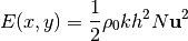
for the energy flux per unit area, , where  are
the wavenumber and amplitude that characterize the bathymetry, and
are
the wavenumber and amplitude that characterize the bathymetry, and
 is the barotropic tidal velocity vector. The
topographic roughness,
is the barotropic tidal velocity vector. The
topographic roughness,  , is derived from the high-resolution
bathymetry ETOPO2v2 (Smith and Sandwell 1997; NGDC 2006)) as the
root-mean-square of the topography over a 50km smoothing radius, and
is a free parameter set as
, is derived from the high-resolution
bathymetry ETOPO2v2 (Smith and Sandwell 1997; NGDC 2006)) as the
root-mean-square of the topography over a 50km smoothing radius, and
is a free parameter set as
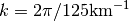 . It should be emphasized that
internal wave conversion equation is a scale relation, and not a precise
specification of internal tide energy-flux. In the barotropic tidal
model, the value of was tuned to give the best fit to the
observed tides.
. It should be emphasized that
internal wave conversion equation is a scale relation, and not a precise
specification of internal tide energy-flux. In the barotropic tidal
model, the value of was tuned to give the best fit to the
observed tides.
9. Other Model Physics
9.1. Equation of State
POP requires an equation of state in the form
(223)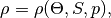
to relate density, , to the prognostic variables
and ; see (10). To avoid a nonlinear
integration of the hydrostatic equation (9), the
pressure, , in the equation of state is approximately evaluated
as a time-independent function of depth  by means of the
equation
by means of the
equation
(224)¶![\begin{aligned}
p_{_0}(z) = 0.059808[\mathrm{exp}(-0.025z)-1]
+0.100766z + 2.28405\times 10^{-7}z^2,
\end{aligned}](../_images/math/d8a198481fd8a9c849727a16bc5946aae8575f3b.png)
where pressure is in bars and depth is in meters.
This formula is derived in Dukowicz (2001) from the latest Levitus
global mean climatology. At a number of places in the code partial
derivatives of with respect to and
may also be necessary.
There are four options in the code for the equation of state:
(A) The density may be obtained from the formula of Jackett and McDougall (1995).
(225)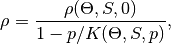
The numerator,  , is a 15-term equation in powers
of and with coefficients given by the UNESCO
international standard equation of state (Fofonoff and Millard 1983).
The secant bulk modulus,
, is a 15-term equation in powers
of and with coefficients given by the UNESCO
international standard equation of state (Fofonoff and Millard 1983).
The secant bulk modulus,  , is a 26-term equation in
powers of , and , obtained from a
least-squares fit to the expression for the secant bulk modulus as a
function of the in situ temperature (Fofonoff and Millard 1983). This
density equation is valid in the range
, is a 26-term equation in
powers of , and , obtained from a
least-squares fit to the expression for the secant bulk modulus as a
function of the in situ temperature (Fofonoff and Millard 1983). This
density equation is valid in the range  ,
,
 , and
, and
 . The total of 41 terms in this equation of
state makes it the most expensive of the four available options.
. The total of 41 terms in this equation of
state makes it the most expensive of the four available options.
(B) A cubic polynomial fit to the UNESCO international standard equation of state (Fofonoff and Millard 1983) which has the form
(226)
where  and
and  are reference
values of the potential temperature and salinity for each model level.
The set of nine coefficients in the cubic polynomial for each level are
pre-calculated based on a least-squares fit to the international
standard equation of state as prescribed by Bryan and Cox (1972). The
range of validity of this equation is depth dependent and is specified
during the fitting procedure to encompass typically observed
oceanographic conditions. This results in a fairly narrow range of
validity at depth which may not be appropriate for certain simulations
or for evaluating density resulting from large adiabatic displacements.
The reduction from 41 terms to 9, however, represents a considerable
cost savings over the full UNESCO equation of state.
are reference
values of the potential temperature and salinity for each model level.
The set of nine coefficients in the cubic polynomial for each level are
pre-calculated based on a least-squares fit to the international
standard equation of state as prescribed by Bryan and Cox (1972). The
range of validity of this equation is depth dependent and is specified
during the fitting procedure to encompass typically observed
oceanographic conditions. This results in a fairly narrow range of
validity at depth which may not be appropriate for certain simulations
or for evaluating density resulting from large adiabatic displacements.
The reduction from 41 terms to 9, however, represents a considerable
cost savings over the full UNESCO equation of state.
(C) A 25-coefficient approximation of the Feistel and Hagen (1995) equation of state (which is more accurate relative to laboratory data than the UNESCO form), derived by McDougall et al. (2003).
(227)
where  is a 12 term polynomial and
  is a 13-term
polynomial. This density equation is valid in the range
is a 13-term
polynomial. This density equation is valid in the range
 ,
,  ,
at the surface, diminishing to
,
at the surface, diminishing to  ,
,
 at 550 bar. However, the
authors report that the equation is well behaved in the range
at 550 bar. However, the
authors report that the equation is well behaved in the range
 ,
,
 , and
This equation of state is intermediate in
cost between the UNESCO form (A) and the cubic polynomial form (B). It
is currently the preferred option for CCSM integrations. An updated form
of this equation of state Jackett et al. (2006) has been implemented in
a future version of POP and should be available soon.
, and
This equation of state is intermediate in
cost between the UNESCO form (A) and the cubic polynomial form (B). It
is currently the preferred option for CCSM integrations. An updated form
of this equation of state Jackett et al. (2006) has been implemented in
a future version of POP and should be available soon.
- A simple linear equation of state given by
(228)
where is in gm/cm , is in
C, and is in practical salinity units (psu).
The term is not included in the code for the full
density with the linear EOS.
, is in
C, and is in practical salinity units (psu).
The term is not included in the code for the full
density with the linear EOS.
9.1.1. Boussinesq Correction
The pressure gradient terms in the momentum equations (44) and
(45) are an approximation of  , introduced
as part of the Boussinesq approximation. Furthermore, the conversion of
pressure to depth in the equation of state by means of (224) can have
significant dynamic consequences through its effect on the pressure
gradient (Dewar et al. 1998). Both of these errors can be greatly
reduced by transforming the density as follows (Dukowicz 2001):
, introduced
as part of the Boussinesq approximation. Furthermore, the conversion of
pressure to depth in the equation of state by means of (224) can have
significant dynamic consequences through its effect on the pressure
gradient (Dewar et al. 1998). Both of these errors can be greatly
reduced by transforming the density as follows (Dukowicz 2001):
(229)
where  is termed the thermobaric density, and
is a nondimensional function of pressure that extracts the
pressure-dependent part of the adiabatic compressibility from the
density along the global-mean Levitus climatology:
is termed the thermobaric density, and
is a nondimensional function of pressure that extracts the
pressure-dependent part of the adiabatic compressibility from the
density along the global-mean Levitus climatology:
(230)
where is in bars. This leads to the definition of an
associated thermobaric pressure  :
:
(231)
such that the hydrostatic equation (9) becomes
(232)
and the pressure gradient force is transformed into
(233)
The effective equation of state in terms of these new variables becomes
(234)
The advantage of this transformation is that the effective adiabatic compressibility associated with the equation of state is now at least an order of magnitude lower. This means that the variation of density with depth is much lower and that fluctuations of pressure in the equation of state have a much smaller effect on density. Thus, the errors associated with the Boussinesq approximation in the pressure gradient force and the linearization of the equation of state in the transformed variables are at least an order of magnitude smaller than without the transformation, as explained in Dukowicz (2001).
The pressure gradient force is approximated by
 , and the hydrostatic equation becomes
(235)
This implies that the pressure variable handled in POP is the
thermobaric pressure , not . The pressure enters
only in the pressure gradient and in the equation of state and effects
nothing else. Should the true pressure ever be required it is easily
obtainable from using the relation (231). Given this, we
shall drop the notation and henceforth interpret
to imply the thermobaric pressure.
9.1.2. Hydrostatic Pressure
The pressure at depth is obtained by integrating the
hydrostatic equation from (the “hydrostatic pressure”
 ) and adding the contribution from the surface pressure
 associated with undulations of the free surface:
(236)
In the code only the horizontal pressure gradients are needed, and these
are evaluated by integrating the horizontal gradients of density in
(236). The discrete formulas for the horizontal pressure
gradients at level are:
(237)¶![\begin{aligned}
&&\delta_x\overline{p_k}^y = \delta_x\overline{p_s}^y
+ g\sum_{m=1}^{k}\frac{1}{2}[\delta_x\overline{\rho^{*}_{m-1}}^y
+\delta_x\overline{\rho^{*}_m}^y]dz_{m-\frac{1}{2}}
\nonumber\\
&&\delta_y\overline{p_k}^x = \delta_y\overline{p_s}^x
+ g\sum_{m=1}^{k}\frac{1}{2}[\delta_y\overline{\rho^{*}_{m-1}}^x
+\delta_y\overline{\rho^{*}_m}^x]dz_{m-\frac{1}{2}}
\end{aligned}](../_images/math/0f5ee35003723ba76ce45dfb3ca26f77cf1e682b.png)
where  , and
, and
 . Here
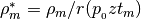 if the Boussinesq correction
is used, otherwise
if the Boussinesq correction
is used, otherwise  , where
  is
the density at level , and
is
the density at level , and  when
when
 .
.
9.1.3. Expansion Diagnostic
This is a feature that is currently not in the code but will be added later. The expansion diagnostic is supposed to account for the change in global mean sea level due to two effects: 1) the change in volume associated with the net accumulated freshwater flux into the ocean (from precipitation, evaporation, melting and freezing of sea ice, and river runoff); and 2) the change in volume associated with steric expansion due to changes in global mean density. If the model employs virtual salinity fluxes, either from restoring to climatological surface salinity or from the conversion of actual freshwater fluxes to virtual salinity fluxes (e.g., when the model is run without using the natural boundary conditions for freshwater flux as discussed in Sec. Variable-Thickness Surface Layer) then the expansion effects due to 1) and 2) are not easily separated: a virtual salinity flux will change the salinity and hence the density through the equation of state, on the other hand, a virtual salinity flux is usually associated with an actual freshwater flux which changes the volume as well, and it is not clear how to cleanly separate these volume and density changes. However, in the steric effect the change in density is primarily associated with thermal expansion due to heating or cooling, rather than changes in salinity. Hence, we expect that computing the steric effect due to density changes without including volume changes due to freshwater flux provides a useful diagnostic. Therefore, in the code the change in surface elevation due to the steric effect can be computed assuming there is no change in total volume. The change in surface elevation due to steric expansion is computed as:
(238)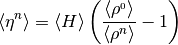
where  , the ratio of ocean volume to surface
area, is the mean ocean depth,
, the ratio of ocean volume to surface
area, is the mean ocean depth,  is the
initial global mean density,
is the
initial global mean density,  is the
global mean density at the
is the
global mean density at the  model timestep
computed assuming there is no change in total volume, and
model timestep
computed assuming there is no change in total volume, and
 is the estimated change in sea-surface
elevation at the timestep due to steric
expansion only. If natural boundary conditions for freshwater flux are
employed, then the actual volume of the ocean in the model does change
(see Sec. Variable-Thickness Surface Layer), and the corresponding change in mean sea
level is diagnosed as the actual global-mean sea level in the model.
This change can be added to the change due to steric expansion to obtain
an approximate total change in global mean sea level due to the combined
effects of 1) and 2).
is the estimated change in sea-surface
elevation at the timestep due to steric
expansion only. If natural boundary conditions for freshwater flux are
employed, then the actual volume of the ocean in the model does change
(see Sec. Variable-Thickness Surface Layer), and the corresponding change in mean sea
level is diagnosed as the actual global-mean sea level in the model.
This change can be added to the change due to steric expansion to obtain
an approximate total change in global mean sea level due to the combined
effects of 1) and 2).
9.2. Sea-Ice Formation and Melting
Air-sea heat fluxes, when applied over a time interval, can produce
regions of subfreezing model upper-layer temperatures. This situation
can be alleviated by adjusting the model and
(and the first layer thickness, if the variable surface thickness
formulation is used with freshwater fluxes) that is associated with
frazil sea-ice formation. The choice of when to perform such adjustments
is judiciously made to ensure tracer conservation with minimum
adjustments. So, in coupled simulations with averaging as the time
mixing option, such ice formation time steps are performed at both the
coupling time step and the time step just prior to it so that both
branches of the leap-frog time steps are brought to the freezing
temperature which will then be used over the next coupling interval. If
Matsuno time mixing option is selected, checking for ice formation
only at the coupling time steps is adequate because the first time step
of the next coupling interval is Matsuno and the unadjusted branch of
the leap-frog time steps will be ignored. The following algorithm
describes the procedure for the virtual salt flux formulation, default
for the present integrations.
After and are updated, the upper kmxice model
layers (denoted by index ) are scanned for below
the freezing point,  . Here, kmxice is a model namelist
input in ice_nml and, at present, is not a function of
local salinity
. Here, kmxice is a model namelist
input in ice_nml and, at present, is not a function of
local salinity  , but
, but  C.
Although we describe the most general case here, in practice we do
recommend setting kmxice=1, because unless a monotone advection scheme
is in place, model advective errors could lead to far
below freezing in some deep locations and the scheme will form too much
ice.
C.
Although we describe the most general case here, in practice we do
recommend setting kmxice=1, because unless a monotone advection scheme
is in place, model advective errors could lead to far
below freezing in some deep locations and the scheme will form too much
ice.
At each layer, the potential mass per unit area of ice melt
 or ice formation
 is computed as
(239)¶![{\tt POTICE}_k = \max \left[ \frac{\rho_{sw} c_p}{L_f}
\Delta z_k (\Theta_f - \Theta_k), {\tt QICE}_{k+1} \right],](../_images/math/ddd2535e1eb735dccf60e2f288f45718aac2b396.png)
where  and
and  are the density and heat
capacity of sea water, respectively, is the latent heat of
fusion,
are the density and heat
capacity of sea water, respectively, is the latent heat of
fusion,  is the layer thickness, and
  is the local potential temperature. Any ice that forms at depth is
assumed to float towards the surface and this ice flux,
is the local potential temperature. Any ice that forms at depth is
assumed to float towards the surface and this ice flux,
 (defined positive downwards so
 ), is accumulated bottom to top as
(240)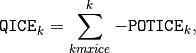
assuming no ice formation below the kmxice layer, i.e.
 . As ice floats to the surface, it can
either partially or completely melt in upper layers whose temperatures
are above freezing.
. As ice floats to the surface, it can
either partially or completely melt in upper layers whose temperatures
are above freezing.
At each layer, and are both adjusted in accord
with the ice formed or melted in the layer:
(241)
For , this is equivalent to replacing a volume of formed ice at
salinity  with an identical volume of water at salinity
 . Here and represent sea ice and
ocean reference salinities, respectively, and they are set to constant
values in order to ensure salt conservation. In addition, if POP is
coupled to a sea-ice model, both must use the same value for
to ensure conservation. Note that in CCSM2,
. Here and represent sea ice and
ocean reference salinities, respectively, and they are set to constant
values in order to ensure salt conservation. In addition, if POP is
coupled to a sea-ice model, both must use the same value for
to ensure conservation. Note that in CCSM2,  , but in CCSM3
 psu.
psu.
The ice flux is accumulated at each location over the number of ice
formation time steps, , during a coupling interval as
(242)
where  is either
  or 1 depending on whether
it is an averaging time step or not.
or 1 depending on whether
it is an averaging time step or not.
If, at the end of a vertical scan, the surface temperature
 remains greater than freezing,
 , then the excess heat melts previously
formed ice, and AQICE, , and
, then the excess heat melts previously
formed ice, and AQICE, , and  are adjusted
accordingly. Thus, over a coupling interval, ice is assumed to remain
where it was formed. In coupled simulations, the accumulated ice during
a coupling interval is passed to an ice model via the flux coupler as an
equivalent downward heat flux, QFLUX in W m
are adjusted
accordingly. Thus, over a coupling interval, ice is assumed to remain
where it was formed. In coupled simulations, the accumulated ice during
a coupling interval is passed to an ice model via the flux coupler as an
equivalent downward heat flux, QFLUX in W m :
:
(243)
where AQICE includes any adjustment due to melting previously formed ice
over the last timestep,  day is the coupling
interval, and
day is the coupling
interval, and  is either or 1 depending on
averaging or Matsuno time steps, respectively. In the last two
equations, the presence of
is either or 1 depending on
averaging or Matsuno time steps, respectively. In the last two
equations, the presence of  s assures that
and budgets will be conserved when the averaging option is
selected where, after averaging, actual and
changes become of what is implied by the ice formation
fluxes.
s assures that
and budgets will be conserved when the averaging option is
selected where, after averaging, actual and
changes become of what is implied by the ice formation
fluxes.
Thus, and adjustments for the total ice formed
 are made prior to the ice being passed to the
sea-ice model. However, warm surface model temperatures result in
are made prior to the ice being passed to the
sea-ice model. However, warm surface model temperatures result in
 , which is a potential to melt ice in the sea-ice
model. Since the ocean does not know if sufficient ice is present at a
given location, and adjustments are delayed
until the appropriate heat and freshwater fluxes are received back from
the sea-ice model through the coupler. If sufficient ice is present in
the absence of all other fluxes, the heat flux will be equal to the
cooling needed to make
, which is a potential to melt ice in the sea-ice
model. Since the ocean does not know if sufficient ice is present at a
given location, and adjustments are delayed
until the appropriate heat and freshwater fluxes are received back from
the sea-ice model through the coupler. If sufficient ice is present in
the absence of all other fluxes, the heat flux will be equal to the
cooling needed to make  , when applied over
the next coupling interval.
, when applied over
the next coupling interval.
The ice formation option can also be activated in ocean-only (uncoupled) simulations subject to observational or reanalysis based air-sea heat fluxes. In this case, the accumulated ice is used internally for local ice formation and melt, and AQICE is saved in restart files for exact continuation. If the Matsuno time step mixing option is chosen, the ice time steps are set to be the time steps just before a mixing step by default. For the averaging time step option, the default is to form ice every time step.
The POP ice formation subroutine contains a modified algorithm when the
freshwater flux formulation is chosen. Here, the volume of ice formed at
layer is replaced with an equal volume of water (because the
thickness of the below surface layers cannot change) from the layer
above with salinity  . The surface layer can
change both through exchanges of with lower layers and change
of thickness due to formed ice sent to the ice model. Because there
still remain some consistencies and scientific issues with ice formation
and melt when freshwater fluxes are used, this algorithm has not yet
been tested, and is not recommended to be used at the present time.
. The surface layer can
change both through exchanges of with lower layers and change
of thickness due to formed ice sent to the ice model. Because there
still remain some consistencies and scientific issues with ice formation
and melt when freshwater fluxes are used, this algorithm has not yet
been tested, and is not recommended to be used at the present time.
9.3. Freshwater Balancing over Marginal Seas
Unlike the surface heat flux and sea surface temperature, there are no
appreciable feedbacks between the surface freshwater flux and .
This is particularly so in isolated marginal sea regions where the
freshwater fluxes can produce unphysical values throughout the
water column. The situation can be especially severe in coupled
integrations when the marginal sea regions receive river runoff fluxes.
In uncoupled integrations, one obvious remedy is to use restoring
freshwater or salt fluxes instead in these regions where the surface
is restored to some climatological distribution with a
relatively small restoring time scale. In this section, we describe a
more novel approach, particularly designed for coupled integrations.
Here, the amount of excess or deficit of freshwater flux over a marginal
sea is transported to or from its associated active-ocean region, thus
implicitly connecting marginal seas with active ocean and providing a
means for marginal sea runoff to eventually discharge into the open
ocean. This process assures that the volume-mean stays
constant throughout the integration within each marginal sea,
eliminating any unphysical values in .
When balancing is requested, the active-ocean regions corresponding to
each marginal sea,  , are determined at the beginning of each
integration. For this computation, a longitude, a latitude (both in
degrees), and a distribution active-ocean area size (in cm)
are provided for each region in an input file. Using the longitude and
latitude values as starting points, a search window is created to find
the active-ocean points associated with each . This iterative
process continues until the cumulative active-ocean grid areas match the
input distribution size. At each iteration, the search window is
increased by 1 on all four sides. If the hard-coded
values for either the maximum number of iterations or the maximum number
of active-ocean grid points per are exceeded, POP will stop
with an error message.
, are determined at the beginning of each
integration. For this computation, a longitude, a latitude (both in
degrees), and a distribution active-ocean area size (in cm)
are provided for each region in an input file. Using the longitude and
latitude values as starting points, a search window is created to find
the active-ocean points associated with each . This iterative
process continues until the cumulative active-ocean grid areas match the
input distribution size. At each iteration, the search window is
increased by 1 on all four sides. If the hard-coded
values for either the maximum number of iterations or the maximum number
of active-ocean grid points per are exceeded, POP will stop
with an error message.
The final product of this initialization procedure is a global array of
area fractions for each ,  . In ,
the fractions are computed simply as the ratios of grid areas to the
total computed distribution area. It is ensured that the sum of these
area fractions for each is unity. The distribution regions
for different can coincide. Note that, the zero elements of
represent the ocean points outside of the designated regions.
. In ,
the fractions are computed simply as the ratios of grid areas to the
total computed distribution area. It is ensured that the sum of these
area fractions for each is unity. The distribution regions
for different can coincide. Note that, the zero elements of
represent the ocean points outside of the designated regions.
In fully coupled integrations in which the surface fluxes stay constant
until the next coupling, balancing is performed once per coupling
interval, immediately following the arrival of the new fluxes. If the
fluxes do change during a coupling interval (e.g. partially-coupled
option), then balancing is done every time step. For each , a
transport term, , is evaluated in Kg s of
freshwater:
(244)¶![\begin{aligned}
T^{ms} = \sum_{ms} \bigl( \bigl[ & \max(0,{\tt QFLUX}_{i,j})c_q + \\
& (E_{i,j} + P_{i,j} + R_{i,j} + M_{i,j}) + F_{i,j}^S c_s \bigr]
\Delta x_{i,j} \Delta y_{i,j} \bigr), \nonumber\end{aligned}](../_images/math/f79b67a31669595a606192ce423317bc1f4e469d.png)
where only the fluxes over the marginal seas contribute to the sum which
is performed over each individually. In the above equation,
 is the frazil ice formation in W
m and , , , and
is the frazil ice formation in W
m and , , , and  represent the evaporation, precipitation, river runoff, and ice melt
freshwater fluxes from the coupler in Kg m
s.
represent the evaporation, precipitation, river runoff, and ice melt
freshwater fluxes from the coupler in Kg m
s.  is the salt flux due to ice melt in Kg of
salt m s. was zero in the
CCSM2 because , but is nonzero in the CCSM3 because
psu in the later version. Finally,
is the salt flux due to ice melt in Kg of
salt m s. was zero in the
CCSM2 because , but is nonzero in the CCSM3 because
psu in the later version. Finally,  and
and
 are the zonal and meridional grid spacings (in m)
centered at points, respectively, and
are the zonal and meridional grid spacings (in m)
centered at points, respectively, and  and
and
 represent unit conversion factors given by
(245)
 represents the excess (or deficit) freshwater flux for
marginal sea that needs to be transported to or from its
associated active-ocean region. How much of is
transported to or from an active-ocean grid point is determined by
represents the excess (or deficit) freshwater flux for
marginal sea that needs to be transported to or from its
associated active-ocean region. How much of is
transported to or from an active-ocean grid point is determined by
(246)
At these points, the surface freshwater or salt flux is modified as
(247)
where  or
or  depending on if POP
is forced with virtual salt or freshwater flux boundary conditions,
respectively.
depending on if POP
is forced with virtual salt or freshwater flux boundary conditions,
respectively.
In marginal seas where there is no frazil ice formation, the surface
freshwater flux is set to zero. Otherwise, the surface flux is simply
computed as  to undo the
adjustment that has been done in the previous time steps.
to undo the
adjustment that has been done in the previous time steps.
Because this algorithm has not yet been used with the freshwater flux formulation, its use is not recommended with that formulation.
9.4. Overflow Parameterization
A new overflow parameterization (OFP) for deep channel overflows (e.g., Denmark Strait and Faroe Bank Channel) and continental shelf overflows (e.g., Weddell and Ross Sea) has been developed and implemented in POP. Although this OFP is based on the Price and Yang (1998) Marginal Sea Boundary Condition (MSBC) scheme, there are substantial differences between the two. The OFP consists of two parts: i) calculation of the overflow properties based on the evolving ocean model state, and ii) modifications of the model boundary conditions, equations, and bottom topography to incorporate the overflow volume and tracer fluxes as well as to ensure volume and tracer conservations. The first part uses the same exchange and entrainment formulas as in the MSBC, but all the necessary fields are obtained prognostically. Furthermore, the marginal seas providing the overflow source waters (e.g., the Nordic Sea) are a part of the prognostic model domain rather than just some marginal sea boundary conditions as in the MSBC and the inflow into these marginal seas is accomplished by the resolved flow in contrast with a parameterized inflow in the MSBC. The second part of the OFP is entirely new, particularly in its treatment of the baroclinic and barotropic momentum and continuity equations to conserve volume.
In POP, overflows can be activated in either interactive or diagnostic mode, where the latter computes the overflow without affecting the model solution. The OFP is used to represent the Denmark Strait, Faroe Bank Channel, Ross Sea, and Weddell Sea overflows. When the overflow module is used either in active or passive mode, the model requires an input file to specify all the details of each overflow region (Briegleb, Danabasoglu, and Large 2010). We note that the OFP is not used to represent the Mediterranean overflow through the Strait of Gibraltar. Instead, we use an open Gibraltar Strait and a sufficiently deep model topography on the Atlantic side of the strait, so that the overflow can convect as deeply as needed locally. This configuration avoids the excess entrainment associated with staircase topography (Wu, Danabasoglu, and Large 2007).
The OFP and its implementation in POP are detailed in Briegleb, Danabasoglu, and Large (2010) and Danabasoglu, Large, and Briegleb (2010), so only a general overview is described here. A schematic of the Nordic Sea overflows and its parameterization are shown in Figure8.1 to help with the following description. For the same purpose, Figure8.2 gives the bottom topography of the model in the vicinity of the Nordic Sea overflows, including the lateral extents of the tracer averaging regions and the pre-specified locations of the possible injection sites for the product waters.
Figure 8.1: A schematic of the Nordic Sea overflows. , ,
, and represent potential temperature,
salinity, density, and volume transport, respectively. The subscripts
, , , and indicate inflow,
source, entrainment, and product water properties, respectively.
is depth,  is the distance from the sill to
the shelf break, is the maximum slope of the
continental shelf near the shelf break,
is the distance from the sill to
the shelf break, is the maximum slope of the
continental shelf near the shelf break,  is the bottom
drag coefficient,
is the bottom
drag coefficient,  is the width of the channel at the sill
depth, and
is the width of the channel at the sill
depth, and  is the upstream thickness of the source water.
The question marks denote the prespecified product water injection
locations. The thick, short arrows indicate flow directions. The
green box shows the raised bottom topography. The other boxes
represent the regions whose and are used to
compute the necessary densities.
is the upstream thickness of the source water.
The question marks denote the prespecified product water injection
locations. The thick, short arrows indicate flow directions. The
green box shows the raised bottom topography. The other boxes
represent the regions whose and are used to
compute the necessary densities.
Figure 8.2: Bottom topography as represented in the model in the vicinity of the Denmark Strait (DMS) and Faroe Bank Channel (FBC) overflows. The colors indicate the model vertical levels. The corresponding depths are given above the color bar. The boxed regions denoted by I, E, and S indicate the Inflow, Entrainment (thin box), and Source regions in the horizontal, respectively, whose potential temperature and salinity properties are used to compute the necessary densities. The source and entrainment box edges at which the respective water properties and transports are imposed as side boundary conditions in the model are indicated by the black arrows, showing directions corresponding to flows out of the model domain. The white lines denoted by P show the prespecified product water injection locations into the model domain. All product water sites have the same injection direction as denoted by the white arrows drawn at only a few of the sites for clarity.
9.4.1. Calculation of Overflow Properties
We use the subscripts , , , and to
denote inflow, source, entrainment, and product water properties,
respectively. In addition to the equations given below, the overflow
dynamics depend on the geography of the straits and channels under
consideration. Here, is the latitude, is the
upstream source thickness, is the width of the strait,
 and
and  are the sill depth and the depth of the
shelf break where entrainment occurs, respectively, is
the distance from the channel exit to the shelf break, is
the maximum bottom slope near the shelf break, and is the
bottom drag coefficient.
are the sill depth and the depth of the
shelf break where entrainment occurs, respectively, is
the distance from the channel exit to the shelf break, is
the maximum bottom slope near the shelf break, and is the
bottom drag coefficient.
The overflows are driven by the density difference between the source
density,  , and the open ocean inflow density,
 , as expressed by the source reduced gravity
(248)
where is the gravitational acceleration and
 kg m is a reference density.
and are evaluated at the sill depth using
kg m is a reference density.
and are evaluated at the sill depth using
(249)
Here, and represent volume-average potential
temperature and salinity, respectively, calculated within the
corresponding horizontal regions shown in Figure8.2 .
There is no averaging in the vertical as only one vertical level is
used.
As long as  source overflow transport will occur.
Assuming that the strait or channel width is greater than the radius of
deformation and the inflow is not geometrically constrained, following
Whitehead, Leetmaa, and Knox (1974), this source overflow transport,
source overflow transport will occur.
Assuming that the strait or channel width is greater than the radius of
deformation and the inflow is not geometrically constrained, following
Whitehead, Leetmaa, and Knox (1974), this source overflow transport,
 , is obtained using the expression for rotating,
hydraulically controlled maximum geostropic flow through a strait
, is obtained using the expression for rotating,
hydraulically controlled maximum geostropic flow through a strait
(250)
It is important to note that (250) uses
( ) which is different than the source thickness above the
sill as the source waters exit the strait, denoted as
) which is different than the source thickness above the
sill as the source waters exit the strait, denoted as  . Again
following Whitehead, Leetmaa, and Knox (1974), is calculated
from as
. Again
following Whitehead, Leetmaa, and Knox (1974), is calculated
from as
(251)
Assuming a rectangular cross sectional area with height and
width , i.e.,  , at the strait exit, an
associated source speed,
, at the strait exit, an
associated source speed,  , can be evaluated
(252)
As the source water flows down along the continental slope, it accelerates, spreads in width, and therefore thins. It also entrains ambient waters in the open ocean, largely near the shelf-slope break. These processes are parameterized using the end-point model of an entraining, rotating density current developed by Price and Baringer (1994). The entrainment is driven by the entrainment reduced gravity given by
(253)
where
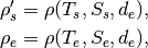
with  and
and  the source and
entrainment region densities, respectively, both computed at the
entrainment depth , using volume-average and
for the corresponding lateral regions shown in
Figure8.2 . As long as
the source and
entrainment region densities, respectively, both computed at the
entrainment depth , using volume-average and
for the corresponding lateral regions shown in
Figure8.2 . As long as  entrainment will occur.
At the shelf break, the flow is assumed to have a characteristic speed governed by geostrophic balance with the reduced gravity flow
(254)
The average flow speed between the channel exit and the shelf break point is then given by
(255)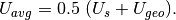
The spreading width is assumed to increase linearly with distance from
the sill such that when the source water reaches the shelf break it has
width  given by
(256)
with the Ekman number,  , specified by the ratio of
bottom drag to Coriolis force over downslope flow
, specified by the ratio of
bottom drag to Coriolis force over downslope flow
(257)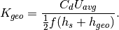
During the lateral spread, the overflow thickness decreases by volume conservation. At the shelf break, the thickness is given by
(258)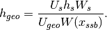
Using (257), (256) and (258) can
be solved simultaneously for  .
.
A geostrophic Froude number,  , for the entrainment mixing
at the shelf-break is defined as
, for the entrainment mixing
at the shelf-break is defined as
(259)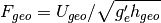
from which an entrainment parameter,  , representing the
ratio of entrained to product water volume transports, can be evaluated
as
, representing the
ratio of entrained to product water volume transports, can be evaluated
as
(260)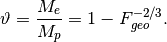
If  or
or  ,
is set to
,
is set to  . Given and , the
entrainment volume transport is
. Given and , the
entrainment volume transport is
(261)
and using volume conservation, the product volume transport is then
(262)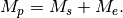
Finally, from tracer conservation, the product water potential temperature and salinity are calculated using
(263)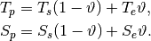
We note that any additional tracers that the model carries, e.g., the
ideal age and CFCs, use the same averaging procedure and conservation
relations as in and .
9.4.2. Model Modifications
As indicated by the green box in Figure8.1 , we raise the
discrete model bottom topography by one vertical level at the sill depth
for each parameterized overflow. This popped-up topography occurs at a
minimum of three consecutive lateral grid points per overflow along the
source water injection site and effectively reduces flow over the sill,
replacing it with the parameterized source flow . These
raised vertical levels represent the only topographic modifications done
when the overflow parameterization is activated compared to the original
topography used in simulations without the OFP. The source flow velocity
and the associated tracer fluxes are imposed as boundary conditions on
the source marginal sea side of the raised level, i.e., at the sill
depth level , as denoted by the blue box in
Figure8.1 . Similarly, the entrainment flow velocity and
tracer fluxes are specified as side boundary conditions on the open
ocean side (Atlantic Ocean in the figure) at the entrainment depth
as shown by the brown box in Figure8.1 . We note
that both the source and entrainment flows are directed into the
topography as indicated by the arrows.
We pre-specify a product water pathway for each overflow, consisting of
 number of possible injection sites as shown by the white
lines in Figure8.2 . To determine where to inject the
product water along this path, we compare the product water density,
number of possible injection sites as shown by the white
lines in Figure8.2 . To determine where to inject the
product water along this path, we compare the product water density,
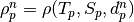 , with the open ocean ambient
water density evaluated at the same depth
, with the open ocean ambient
water density evaluated at the same depth  , using the
volume-average and from the immediate downstream of
the th product water site. Assuming that the product water
injection site depths monotonically increase with , i.e., the
th site representing the deepest one, our search starts
with the (
, using the
volume-average and from the immediate downstream of
the th product water site. Assuming that the product water
injection site depths monotonically increase with , i.e., the
th site representing the deepest one, our search starts
with the ( )th site and ends at the first one. If
 exceeds the ambient density at level , the
product water is inserted as a lateral boundary condition at the next
deepest site . This process ensures that the product water
goes to the deepest possible site. The injection occurs at the
shallowest site if is never larger than the ambient
density at any of the sites. As shown in Figure8.1 , the
product water is directed out of the bottom topography. In effect, the
flow between source to entrainment and then entrainment to product
occurs below the model bottom topography through the parameterization.
We remark that the ambient ocean density along the product path is not
necessarily monotonically increasing, because the product path extends
laterally as it deepens.
exceeds the ambient density at level , the
product water is inserted as a lateral boundary condition at the next
deepest site . This process ensures that the product water
goes to the deepest possible site. The injection occurs at the
shallowest site if is never larger than the ambient
density at any of the sites. As shown in Figure8.1 , the
product water is directed out of the bottom topography. In effect, the
flow between source to entrainment and then entrainment to product
occurs below the model bottom topography through the parameterization.
We remark that the ambient ocean density along the product path is not
necessarily monotonically increasing, because the product path extends
laterally as it deepens.
The specification of the overflow volume transports as side wall velocity boundary conditions for the source, entrainment, and product sites requires careful modifications of the baroclinic and barotropic equations to ensure local mass (volume) conservation from which the global conservation follows automatically. Here, we repeat some equations for clarity. With baroclinic and barotropic split, the total velocity is written as
(264)
where  and are the
baroclinic and barotropic velocities, respectively. They are defined by
and are the
baroclinic and barotropic velocities, respectively. They are defined by
(265)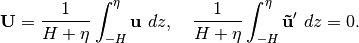
We assume that the injected side wall overflow velocities represent the
total velocity . For those U-grid columns where these
injections occur, must be extended downwards to the bottom of
the vertical grid level where the overflow velocities are actually
specified. This new depth is given by
(266)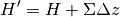
where  denotes the vertical level thicknesses and the
summation is done for the side wall heights from down to the
bottom of the injection level. To avoid complications arising from
moving product water injection locations, we change to
denotes the vertical level thicknesses and the
summation is done for the side wall heights from down to the
bottom of the injection level. To avoid complications arising from
moving product water injection locations, we change to
 at all product water sites. If the
injection level is several vertical grid levels below , the
thicknesses of the levels in between are included in this summation.
These in-between levels are assumed to have
at all product water sites. If the
injection level is several vertical grid levels below , the
thicknesses of the levels in between are included in this summation.
These in-between levels are assumed to have  . Thus, we
replace with in all model equations where
appropriate, including any relevant vertical integrals. For example,
(265) becomes
. Thus, we
replace with in all model equations where
appropriate, including any relevant vertical integrals. For example,
(265) becomes
(267)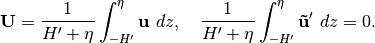
As described earlier, POP first solves the momentum equations, without
including the surface pressure gradient, for an auxiliary velocity
 , giving us between
 . The relationship between this intermediate
velocity and is
. The relationship between this intermediate
velocity and is
(268)
Our assumption of at the side walls between
and any overflow injection levels leads to
 at these in-between levels.
Similarly, because
at these in-between levels.
Similarly, because  , we have
 at all the
injection locations. Here, is a generic
variable used to indicate the overflow velocities. So, knowing
(see below), between
at all the
injection locations. Here, is a generic
variable used to indicate the overflow velocities. So, knowing
(see below), between
 , and between
 , we use (267) and (268)
to obtain an equation for
, we use (267) and (268)
to obtain an equation for  for the
entire column
for the
entire column
(269)¶![{\overline {{\bf u}^{\prime}}} =
\frac{1}{H} \left[ \int_{-H}^\eta {\bf u}^{\prime} ~ dz +
\int_{-H^\prime}^{-H} {\bf \tilde u}^\prime ~ dz \right].](../_images/math/9c89e56ed36cf1dc61e302fdf2b8676b3b51ddca.png)
We then evaluate using (268)
for . This process results in local volume
conservation, consistent with the imposed overflow velocities, for the
T-grid columns to the immediate upstream (to the right in
Figure8.1 ) of the source and to the immediate downstream
(to the left in Figure8.1 ) of the entrainment and product
injection locations.
These velocity modifications obviously impact the horizontal velocity divergences, thus destroying the local volume conservation, at the T-grid columns immediately downstream (to the left in Figure8.1 ) of the source and immediately upstream (to the right in Figure8.1. ) of the entrainment and product injection sites. For example, the T-grid column above the raised sill has a non-zero vertical velocity at the bottom of the column. The magnitudes of these imbalances are equal to the volume transports associated with the source, entrainment, and product waters for each affected column. Therefore, we modify the vertically integrated continuity equation for these columns to account for these transports and thus enforce continuity, viz.,
(270)
where  is 1 for the affected columns and 0
elsewhere,
is 1 for the affected columns and 0
elsewhere,  represents either ,
  ,
or
,
or  , and
, and  is the appropriate surface area of
the affected T-grid columns. (270) together with the
vertically integrated momentum equation are then used to compute both
and . It is important to reiterate here that
the last term on the left-hand side of (270) accounts for the
changes in the horizontal velocity divergences within a specified T-grid
column and it should not be viewed as mass (volume) injections /
extractions from either the surface or the ocean bottom.
is the appropriate surface area of
the affected T-grid columns. (270) together with the
vertically integrated momentum equation are then used to compute both
and . It is important to reiterate here that
the last term on the left-hand side of (270) accounts for the
changes in the horizontal velocity divergences within a specified T-grid
column and it should not be viewed as mass (volume) injections /
extractions from either the surface or the ocean bottom.
The changes in the tracer equations are relatively straightforward compared to the momentum equations. Specifically, the advection algorithms are modified to incorporate the non-homogeneous flux boundary conditions at the injection sites. By construction, this process conserves all tracers. For further details, see Briegleb, Danabasoglu, and Large (2010).
9.5. Passive Tracers
Passive tracers are defined as tracers that do not impact the physical solution, but are carried along with the flow with perhaps some internal transformations that do not feed back on the prognostic tracer. POP contains a tracer infrastructure that accommodates such tracers. Two examples are described here that provide diagnostics for the age of ocean water and long term transport.
9.5.1. Ideal Age
Ideal age is a tracer used to estimate ventilation timescales in the ocean (Thiele and Sarmiento 1990; England 1995). Ideal age satisfies the same tracer transport equation as potential temperature and salinity, e.g., equations (11) and (34), but with different surface boundary conditions. In particular, ideal age is set to zero in the model surface layer at each time step. In startup runs, ideal age is initialized to zero everywhere.
Each water parcel ages by one year for each year since last contact with the surface ocean. In practice, ideal age is incremented by the model time step at each time step. The only way that indefinite growth of ideal age is limited is by contact with the surface, or by mixing with waters that have recently contacted the surface. The oldest ages will be found in waters which have been removed from the surface for the longest period of time. Ideal age equilibrates to its steady state solution on a timescale of thousands of years. The ocean model carries ideal age as a default tracer, and it is reported in units of years.
9.5.2. Chlorofluorocarbons
Chlorofluorocarbons (CFCs) are non-toxic chemicals containing chlorine, carbon, and fluorine atoms. They were developed in the early 1930s and widely used as refrigerants, in aerosol applications, and as solvents. Their concentration increased in the atmosphere until it was recognized that they contribute to ozone depletion in the stratosphere, and they began to be phased out by the Montreal Protocol in the late twentieth century. CFCs enter the ocean via air-sea gas exchange with the atmosphere. Both CFC-11 and CFC-12 are inert in seawater, and have been widely measured throughout the world ocean in the late 20th century and early 21st century. CFCs provide a useful diagnostic for timescales and pathways of transport in ocean models (Dutay et al. 2002) because they can be directly compared against observations.
In POP, surface CFC fluxes are calculated from 1931.5 through 2008.5,
largely following OCMIP 2 protocols (OCMIP 2000). However, instead of
using the atmospheric fields specified by OCMIP, atmospheric datasets
for 10m winds, atmospheric pressure and ice fraction are used in
computing the air-sea CFC flux. Values specified for the atmospheric CFC
partial pressure (pCFC) history up to 1998.5 are from OCMIP 2. Values
from 1999.5 on are from Walker, Weiss, and Salameh (2009). Values were
extended from 1999.5 to 2008.5 by converting from SIO-1998 scale to
SIO-1993 scale in order to be consistent with pre-1998 values. Both
CFC-11 and CFC-12 are reported in units of
 (which is within a few percent of
pmol/kg).
(which is within a few percent of
pmol/kg).
10. Forcing
Most of the surface forcing is implemented as a surface flux and applied as the flux across the top face in vertical mixing routines. The remaining details pertain to which fields are required and the options are covered in the POP User’s Guide. Here we describe the solar radiative forcing and some conservation details that require more description.
10.1. Penetration of Solar Radiation
POP contains several options for allowing solar radiation to penetrate the water column.
10.1.1. Jerlov Water Type
One form of this absorption allows the user to specify a Jerlov water
type. This assumption for solar absorption has the form of a double
exponential, with the fraction of surface shortwave solar radiation,
 , that reaches a depth,
  , given by :
(271)
The first term on the right-hand side represents the rapid absorption of
the longer wavelengths (reds), so the extinction  is small
(
is small
( m) and a fraction
(
m) and a fraction
( ) of the radiation is in this band. The
extinction
) of the radiation is in this band. The
extinction  for the shorter wavelengths (blues) is much
greater (
for the shorter wavelengths (blues) is much
greater ( m). These parameters are set
according to a specific Jerlov water type, and are varied neither
spatially, nor in time. An important restriction is that no solar
radiation passes through the bottom of the model ocean, lest it be lost
to the system. Also, in order to avoid numerical underflows associated
with vanishingly small exponentials,
m). These parameters are set
according to a specific Jerlov water type, and are varied neither
spatially, nor in time. An important restriction is that no solar
radiation passes through the bottom of the model ocean, lest it be lost
to the system. Also, in order to avoid numerical underflows associated
with vanishingly small exponentials,  for depths deeper
than
for depths deeper
than  . Jerlov water type Ib is typical.
10.1.2. Absorption Based on Chlorophyll
Another option in POP activates a chlorophyll dependent solar absorption
that is based on the parameterization of Ohlmann (2003). Its form is a
double exponential, with the transmission from surface to depth,
, given by:
(272)
When this transmission is multiplied by the net shortwave absorption of
the entire column; i.e. down shortwave at surface times one minus ocean
albedo, there results the net flux transmitted to depth, , for
a given chlorophyll amount. The A,B coefficients are chlorophyll
dependent. The effects of solar zenith angle and cloud amount are small,
and are ignored in the present implementation. Chlorophyll is assumed to
be uniformly distributed in the column. As with the Jerlov-based
transmission, no solar radiation passes through the bottom of the model
ocean. Chlorophyll amounts range from  for pure
ocean water, to
for pure
ocean water, to  in chlorophyll blooms.
Transmissions are estimated to be accurate to
in chlorophyll blooms.
Transmissions are estimated to be accurate to  .
.
For this option, the user must specify the chlorophyll amount in an
input data file. This file contains twelve monthly chlorophyll amounts
in  on the ocean horizontal grid. The monthly
chlorophyll distributions were provided by Ohlmann, based on a limited
set of SeaWIFS data spanning the period September 1997 to November 2001.
Regional values range from
on the ocean horizontal grid. The monthly
chlorophyll distributions were provided by Ohlmann, based on a limited
set of SeaWIFS data spanning the period September 1997 to November 2001.
Regional values range from  typical of subtropical
oceans far from continents, to mid-latitude, coastal and equatorial
values from
typical of subtropical
oceans far from continents, to mid-latitude, coastal and equatorial
values from  to
to  . A few coastal
regions have bloom values of .
. A few coastal
regions have bloom values of .
Transmissions vary spatially and are updated once a month, with a
repeating annual cycle. Chlorophyll based transmissions are nearly the
same as the standard Jerlov water type Ib transmissions for a
chlorophyll amount of  . Generally, the subtropical
oceans away from continents have more transmissive surface layers than
the Jerlov case, while midlatitude, coastal and equatorial surface
layers are less transmissive.
. Generally, the subtropical
oceans away from continents have more transmissive surface layers than
the Jerlov case, while midlatitude, coastal and equatorial surface
layers are less transmissive.
10.1.3. Diurnal Cycle
Because POP is often run in situations where it receives only daily shortwave fluxes, there are three options for specifying how the net shortwave flux is distributed in time to mimic a diurnal cycle. The first option keeps the spatially varying flux constant for the duration of the coupling interval.
The second option distributes the flux across a 12 hour window centered at noon. Inside this window, the flux is proportional to a sine term. The flux is zero outside of this window. The distribution is normalized to conserve the integral of the shortwave flux over the coupling interval. This option, whose impact is described in Danabasoglu et al. (2006), works only when the coupling frequency is once per day. Note that the sine distribution curve is independent of longitude, latitude, and time of year.
In the third option, the flux is proportional to the cosine of the solar zenith angle. The distribution is normalized to conserve the integral of the shortwave flux over the coupling interval. This option can be used with any coupling frequency. The solar zenith angle is determined from longitude, latitude, time of year, and the solar declination angle, which is determined from orbital parameters passed from the flux coupler. The zenith angle and declination angle computations make use of CCSM shared code.
10.2. Ice Runoff
In CCSM4, the ocean model receives an ice runoff field,  , in
addition to the liquid water runoff, . To conserve heat in the
coupled system, the associated phase change is accounted for in POP by
adding the latent heat,
, in
addition to the liquid water runoff, . To conserve heat in the
coupled system, the associated phase change is accounted for in POP by
adding the latent heat,  , to the total ocean surface heat
flux. The freshwater flux due to total runoff is then
, to the total ocean surface heat
flux. The freshwater flux due to total runoff is then  .
.
10.3. Tracer Fluxes and Averaging Time Steps
In coupled applications it is essential that an accurate accounting of tracer fluxes through the sea surface be maintained in order to allow for conservative exchange within the full coupled system. The use of a leapfrog scheme, with its even and odd branches, presents some complexity in this respect, and the use of averaging steps to suppress the leapfrog computational mode (Section Filtering Timesteps) must also be taken into account.
We consider our accounting problem over a coupling interval, defined by successive times of information exchange between ocean model and coupler. It is sufficient to consider the use of a single averaging step within that interval, but with the restriction that none of the three time levels which are to be averaged fall outside of the coupling interval. We note that this implies that the last time step prior to a coupling time step is always a leapfrog time step.
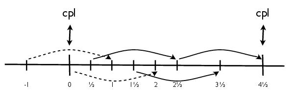
Figure 9.1: Illustration of a coupling interval containing a single averaging step, with cpl identifying times at which information is exchanged with the coupler (time advances to the right). Steps taken before averaging are represented with dashed lines, steps taken after averaging are represented with solid lines.
The illustration presented in Figure9.1 includes
five leapfrog steps within the coupling interval from time to
time  . To streamline notation here we consider
only the influence of the surface flux on the leapfrog
evolution of , omitting the reference point
from the time index and the geometric factors which would multiply the
surface flux. Considering only the tendency due to surface fluxes then
the tracer evolution of the two leapfrog branches begins with
. To streamline notation here we consider
only the influence of the surface flux on the leapfrog
evolution of , omitting the reference point
from the time index and the geometric factors which would multiply the
surface flux. Considering only the tendency due to surface fluxes then
the tracer evolution of the two leapfrog branches begins with
(273)
An averaging step is then applied to time levels ,  and
and  in order to suppress the leapfrog computational mode
(Section Filtering Timesteps):
in order to suppress the leapfrog computational mode
(Section Filtering Timesteps):
(274)
We resume ordinary leapfrog timestepping, still using information
exchanged at the beginning of the coupling interval, until we have
produced  , the tracer at the end of the
coupling interval:
, the tracer at the end of the
coupling interval:
(275)
Summing (273) and (275), and making use of (274), the change in the average of the leapfrog branches over the coupling interval may be expressed in terms of the fluxes which span the coupling interval, as
(276)
We accurately account for the fluxes passing through the ocean surface based on this expression, with the exception of the very first coupling interval of a run which starts with a forward step, as in initial startup from climatology (we permit this one-time departure from strict conservation).
Under current practice, at the time this document is being prepared, the only temporal variation which may occur within the fluxes spanning a coupling interval is due to the use of an idealized diurnal cycle (Section Penetration of Solar Radiation), and due to the latent heat associated with the formation or melting of ice. The idealized diurnal cycle is conservative and used only when coupling is daily. It does not change the amount of incoming SW, but only its temporal distribution. Ice formation is only considered at the time of coupling, at which point both branches of the leap-frog time steps are modified, as explained in Section Sea-Ice Formation and Melting, resulting in the addition of the QFLUX term of (243) to the right hand side of (276).
If another method of controlling the leapfrog computational mode is to be used then the accounting of fluxes must be reconsidered. With use of Matsuno steps an exact accounting is straightforward. An exact accounting of fluxes is more problematic with use of a Robert-Asselin time filter, as discussed in Leclair and Madec (2009).
11. Parallel Implementation
POP has been designed to run effectively on a wide variety of high performance computing architectures. It has also been designed for portability, so that no changes in the code itself are required to compile and run on a new architecture. This has been achieved by adhering to language standards and by abstracting communication functions to support multiple messaging or other communication paradigms. No preprocessing directives are used, except to maintain some differences between the CCSM version and the standalone POP, primarily due to coupling and CCSM shared code issues. In this chapter, details of the domain decomposition algorithms, the communication architecture and parallel I/O are described. Instructions on configuring POP inputs for performance are included in the POP User’s Guide.
11.1. Domain Decomposition
In order to compute efficiently on parallel architectures, work must be divided among each distributed computing node. POP, like many other climate or fluid dynamics models, achieves this parallelism through domain decomposition, dividing the gridded domain into pieces that each node can compute relatively independently. To increase this independence, ghost cells or halo regions are defined so that a node will have some information about state variables on neighboring nodes (see Figure10.1 ). This enables the calculation on each node to proceed without communicating with other nodes until these regions need to be updated. In POP, using a halo width of two grid cells will ensure that the entire baroclinic tendencies can be computed without any inter-node communication.
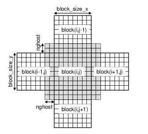
Figure 10.1: An illustration of a ghost cell or halo region, showing the halo for a particular block based on neighboring blocks.
Originally, POP decomposed the domain into single blocks per node. From POP 2.0 onward, POP has used a more flexible decomposition. In the new decomposition, the horizontal domain continues to be divided into blocks, but multiple blocks can be distributed to each node, as shown in Figure10.2a , Figure10.2b , Figure10.2c , Figure10.2d . This structure enables the optimization of block size for cache performance. Multiple blocks on a node also provides a mechanism for hybrid parallelism, in which a threaded parallelism (e.g. OpenMP) can be used to distribute work within a multi-processor shared memory node, while message passing (e.g. MPI) is still used to communicate between distributed nodes. Furthermore, different numbers of blocks can be assigned to each node to balance the computational load. Finally, this scheme permits the elimination of blocks which contain only land points. Such a structure provides additional optimization tuning flexibility. The use of small blocks can eliminating more land, provide better load balancing and better performance on cache-based microprocessors. However, because each block has a halo region, blocks that are too small have a high surface-to-volume ratio and communication and synchronization issues become dominant. Generally, block sizes of 20-40 grid points in each direction appear to provide a reasonable balance, though each computer is different.
Figure 10.2a: The POP subblocking decomposition, showing the full domain with shaded land cells
Figure 10.2b: The POP subblocking decomposition, showing a traditional single block Cartesian
Figure 10.2c: The POP subblocking decomposition, showing a subblock decomposition
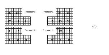
Figure 10.2d: The POP subblocking decomposition, showing a distribution of blocks in which land block have been eliminated and the computational load has been balanced.
POP supports three different schemes for distributing blocks among processors. All of them eliminate land blocks, but each represents options for balancing the number of blocks per node.
11.1.1. Cartesian Distribution
The first option for block distribution is a simple Cartesian distribution. In this case, the sublocks in a domain are distributed according to their logical position in the domain with a two-dimensional rectangular decomposition, similar to that shown in Figure10.2b , except that the single blocks in that figure would correspond to the set of subblocks associated with those large portions of the domain. No load balancing occurs and some nodes may be left with no work to do if all blocks are land.
11.1.2. Rake Distribution
A second distribution scheme uses a simple rake algorithm to balance the work per node. The algorithm starts with the Cartesian distribution described above. Then an average number of blocks per node is computed. In each dimension, the algorithm starts with the first block in that dimension and determines whether the number of blocks exceeds the mean and if so, blocks are passed on to the next node in line. This can be visualized as a rake passing over each node and dragging excess work into the next available “hole”. In POP, additional constraints are placed on block movements, so that if a block is moved once, it is not likely to be moved again and another block is chosen for the move. This attempts to keep neighboring blocks as local as possible. Because the rake is performed in each logical direction separately, there are instances where the algorithm can actually result in a worse load imbalance as blocks get raked into a corner. Also, if there are relatively few blocks per node, load balancing is not very effective.
11.1.3. Space-filling Curve Distribution
A third distribution method is a partitioning algorithm based on
space-filling curves (SFC). This algorithm draws a curve through the set
of blocks in a way that maintains locality and can more effectively
balance both the computational load and the communications costs.
Details can be found in Dennis (2007). While the space-filling curve
algorithm is supported for all resolutions, it is particularly effective
at reducing the cost of high resolution simulations. Use of the SFC
partitioning places restrictions on the size sub-blocks used by POP. In
particular the size of the sub-blocks  and
and
 must be selected under the constraint that
 and
and  are
integers such that
are
integers such that  where
, , and are integers and
where
, , and are integers and  and
and  refer to the global size of the horizontal
computational grid.
refer to the global size of the horizontal
computational grid.
As mentioned above, in addition to improving the computational load balance, SFC partitioning also has a tendency to improve the communication load balance of POP (Dennis 2007). In particular it randomizes network traffic on machines with fixed interconnect topologies, resulting in decreased network congestion and communication time.
11.2. Parallel I/O
In a parallel implementation, the lack of a parallel I/O subsystem creates a serial bottleneck that limits performance. Originally, POP created a parallel I/O system by gathering a single horizontal slice of a 3-D array onto one of the I/O tasks and that task wrote the slice into a specified record of a binary direct-access file. This system was not always robust, due to local machine I/O issues (e.g. system I/O buffers being overwritten by multiple writers) and because this limits the number of I/O tasks and requires each task to keep a full global slice of the data. Finally, this implementation did not support netCDF.
A new parallel I/O library, PIO, has been developed as a collaborative
effort by NCAR/CISL, DOE/SciDAC and NCAR/CSEG. PIO was initially
designed to allow  POP to execute and write history and
restart files on Blue Gene/L using less than 256 MB per MPI task due to
better memory management, relaxing the requirement for retaining a full
global slice on each I/O task.
POP to execute and write history and
restart files on Blue Gene/L using less than 256 MB per MPI task due to
better memory management, relaxing the requirement for retaining a full
global slice on each I/O task.
Since that initial prototype version, PIO has developed into a general purpose parallel I/O library that currently supports netCDF (serial), pnetCDF and MPI_IO and has been implemented throughout the entire CCSM system. PIO is a software interface layer designed to encapsulate the complexities of parallel IO and to make it easier to replace the lower level software backend. PIO calls are collective, an MPI communicator is set in a call to PIO_init and all tasks associated with that communicator must participate in all subsequent calls to PIO.
One of the key features of PIO is that it takes the model’s decomposition and redistributes it to an I/O “friendly” decomposition on the requested number of I/O tasks. In using the PIO library for netCDF or pnetCDF I/O, the user must specify the number of iotasks to be used, the stride or number of tasks between iotasks and whether the I/O will use the serial netCDF or pnetCDF library. By varying the number of iotasks, the user can easily reduce the serial I/O memory bottleneck (by increasing the number of iotasks), even with the use of serial netCDF.
12. References
Adcroft, A., J.-M. Campin, P. Heimbach, C. Hill, and J. Marshall. 2005. MITgcm Manual. http://mitgcm.org/pelican/online\_documents/manual.html.
Adcroft, A., C. Hill, and J. Marshall. 1997. “Representation of Topography by Shaved Cells in a Height Coordinate Ocean Model.” Mon. Wea. Rev. 125: 2293–2315.
Arakawa, A., and V.R. Lamb. 1977. “Computational Design of the Basic Dynamical Processes of the UCLA General Circulation Model.” Methods of Computational Physics 17: 173.
Arfken, G. 1970. Mathematical Methods for Physicists. Academic, New York.
Boccaletti, Giulio, Raffaele Ferrari, and Baylor Fox-Kemper. 2007. “Mixed Layer Instabilities and Restratification.” J. Phys. Oceanogr. 37: 2228–50. doi:10.1175/JPO3101.1.
Briegleb, B.P., G. Danabasoglu, and W.G. Large. 2010. An over Flow Parameterization for the Ocean Component of the Community Climate System Model. NCAR Tech. Note NCAR/TN-xxxx + STR. National Center for Atmospheric Research.
Brown, J.A., and K. A. Campana. 1978. “An Economical Time-Differencing Scheme for Numerical Weather Prediction.” Mon. Weather Rev. 106: 1125–36.
Bryan, K. 1969. “A Numerical Method for the Study of the World Ocean.” J. Comp. Phys. 4: 347–76.
———. 1984. “Accelerating the Convergence to Equilibrium of Ocean-Climate Models.” J. Phys. Oceanogr. 14: 666–73.
Capet, X., E. J. Campos, and A. M. Paiva. 2008. “Submesoscale Activity over the Argentinian Shelf.” Geophysical Research Letters 35. doi:ARTN L15605.
Capet, X., J. C. McWilliams, M. J. Molemaker, and A. F. Shchepetkin. 2008. “Mesoscale to Submesoscale Transition in the California Current System. Part III: Energy Balance and Flux.” J. Phys. Oceanogr. 38: 2256–69. doi:DOI 10.1175/2008JPO3810.1.
Cox, M.D. 1987. “Isopycnal Diffusion in a Z-Coordinate Ocean Model.” Ocean Modelling 74: 1–5.
Danabasoglu, G. 2004. “A Comparison of Global Ocean General Circulation Model Solutions Obtained with Synchronous and Accelerated Integration Methods.” Ocean Modelling 7: 323–41.
Danabasoglu, G., and J. Marshall. 2007. “Effects of Vertical Variations of Thickness Diffusivity in an Ocean General Circulation Model.” Ocean Modelling 18: 122–41, doi:10.1016/j.ocemod.2007.03.006.
Danabasoglu, G., and J. C. McWilliams. 1995. “Sensitivity of the Global Ocean Circulation to Parameterizations of Mesoscale Tracer Transports.” J. Climate 8: 2967–87.
Danabasoglu, G., R. Ferrari, and J.C. McWilliams. 2008. “Sensitivity of an Ocean General Circulation Model to a Parameterization of Near-Surface Eddy Fluxes.” J. Climate 21: 1192–1208, doi:10.1175/2007JCLI1508.1.
Danabasoglu, G., W.G. Large, and B.P. Briegleb. 2010. “Climate Impacts of Parameterized Nordic Sea Overflows.” Submitted.
Danabasoglu, G., W.G. Large, J.J. Tribbia, P.R. Gent, B.P. Briegleb, and J.C. McWilliams. 2006. “Diurnal Coupling in the Tropical Oceans of CCSM3.” J. Climate 19: 2347–65.
Dennis, J. M. 2007. “Inverse Space-Filling Curve Partitioning of a Global Ocean Model.” In Proceedings of IEEE International Parallel and Distributed Processing Symposium.
Dewar, W., Y. Hsueh, T. J. McDougall, and D. Yuan. 1998. “Calculation of Pressure in Ocean Simulations.” J. Phys. Oceanogr. 28: 577–88.
Dukowicz, J. K., R. D. Smith, and R. C. Malone. 1993. “A Reformulation and Implementation of the Bryan-Cox-Semtner Ocean Model on the Connection Machine.” J. Atmos. Ocean Tech. 14: 294–317.
Dukowicz, J.K. 2001. “Reduction of Density and Pressure Gradient Errors in Ocean Simulations.” J. Phys. Oceanogr. 31: 1915–21.
Dukowicz, J.K., and R.D. Smith. 1994. “Implicit Free-Surface Formulation of the Bryan-Cox-Semtner Ocean Model.” J. Geophys. Res. 99: 7991–8014.
———. 1997. “Stochastic Theory of Compressible Turbulent Fluid Transport.” Phys. Fluids 9: 3523–29.
Dutay, J.-C., J. Bullister, S.Doney, J. Orr, R. Naijar, K. Caldeira, J.-M. Campin, et al. 2002. “Evaluation of Ocean Model Ventilation with CFC-11: Comparison of 13 Global Ocean Models.” Ocean Modelling 4: 89–120.
D’Azevedo, E.F., V.L. Eijkhout, and C.H. Romine. 1993. LAPACK Working Note 56. Conjugate Gradient Algorithms with Reduced Synchronization Overhead on Distributed Memory Multiprocessors. Tech. Rep. CS-93-185. Knoxville, TN: Computer Science Department, University of Tennessee.
Eden, C., and R.J. Greatbatch. 2008. “Towards a Mesoscale Eddy Closure.” Ocean Modelling 20: 223–39.
Eden, C., M. Jochum, and G. Danabasoglu. 2009. “Effects of Different Closures for Thickness Diffusivity.” Ocean Modelling 26: 47–59.
England, M. 1995. “The Age of Water and Ventilation Timescales in a Global Ocean Model.” J. of Phys. Oceanogr. 25: 2756–77.
Farrow, D.E., and D.P. Stevens. 1995. “A New Tracer Advection Scheme for Bryan and Cox Type Ocean General Circulation Models.” J. Phys. Oceanogr. 25: 1731–41.
Feistel, R., and E. Hagen. 1995. “On the GIBBS Thermodynamic Potential of Seawater.” Prog. in Oceanogr. 36: 249–327.
Ferrari, R, and D L Rudnick. 2000. “Thermohaline Variability in the Upper Ocean.” Journal of Geophysical Research-Oceans 105: 16857–83.
Ferrari, R, and W R Young. 1997. “On the Development of Thermohaline Correlations as a Result of Nonlinear Diffusive Parameterizations.” Journal of Marine Research 55: 1069–1101.
Ferrari, R., J.C. McWilliams, V.M. Canuto, and M. Dubovikov. 2008. “Parameterization of Eddy Fluxes Near Oceanic Boundaries.” J. Climate 21: 2770–89, doi:10.1175/2007JCLI1510.1.
Ferreira, D., and J. Marshall. 2006. “Formulation and Implementation of a ‘Residual-Mean’ Ocean Circulation Model.” Ocean Modelling 13: 86–107.
Ferreira, D., J. Marshall, and P. Heimbach. 2005. “Estimating Eddy Stresses by Fitting Dynamics to Observations Using a Residual-Mean Ocean Circulation Model and Its Adjoint.” J. Phys. Oceanogr. 35: 1891–1910.
Fofonoff, N.P., and R. C. Millard. 1983. “Algorithms for Computation of Fundamental Properties of Seawater.” UNESCO Technical Papers in Marine Science 44: 53.
Fox-Kemper, B., G. Danabasoglu, R. Ferrari, and R. W. Hallberg. 2008. “Parameterizing Submesoscale Physics in Global Climate Models.” CLIVAR Exchanges 13: 3–5.
Fox-Kemper, B., G. Danabasoglu, R. Ferrari, S. M. Griffies, R. W. Hallberg, M. M. Holland, S. Peacock, and B. L. Samuels. 2010. “Parameterization of Mixed Layer Eddies. III: Global Implementation and Impact on Ocean Climate Simulations.”
Fox-Kemper, Baylor, and Raffaele Ferrari. 2008. “Parameterization of Mixed Layer Eddies. Part II: Prognosis and Impact.” J. Phys. Oceanogr. 38: 1166–79. doi:10.1175/2007JPO3788.1.
Fox-Kemper, Baylor, Raffaele Ferrari, and Robert Hallberg. 2008. “Parameterization of Mixed Layer Eddies. Part I: Theory and Diagnosis.” J. Phys. Oceanogr. 38: 1145–65. doi:10.1175/2007JPO3792.1.
Garrett, C.J.R., and W. H. Munk. 1975. “Space-Time Scales of Internal Waves: A Progress Report.” J. Geophys. Res. 80: 291–97.
Gent, P.R., and J. C. McWilliams. 1990. “Isopycnal Mixing in Ocean Circulation Models.” J. Phys. Oceanogr. 20: 150–55.
Gerdes, R., C. Koberle, and J. Willebrand. 1991. “The Influence of Numerical Advection Schemes on the Results of Ocean General Circulation Models.” Climate Dynamics 5: 211–26.
Gregg, M.C. 1987. “Diapynal Mixing in the Thermocline: A Review.” J. Geophys. Res. 92: 5249–86.
———. 1989. “Scaling Turbulent Dissipation in the Thermocline.” J. Geophys. Res. 94: 9686–98.
Griffies, S.M. 1998. “The Gent-McWilliams Skew Flux.” J. Phys. Oceanogr. 28: 831–41.
Griffies, S.M., and R. W. Hallberg. 2000. “Biharmonic Friction with a Smagorinsky-Like Viscosity for Use in Large-Scale Eddy-Permitting Ocean Models.” Monthly Weather Review 128: 2935–46.
Griffies, S.M., A. Gnanadesikan, R. C. Pacanowski, V. Larichev, J. K.
Dukowicz, and R. D. Smith. 1998. “Isoneutral Diffusion in a
-Coordinate Ocean Model.” J. Phys. Oceanogr. 28: 805–30.
Griffies, S.M., R. C. Pacanowski, M. Schmidt, and V. Balaji. 2001. “Tracer Conservation with an Explicit Free Surface Method for Z-Coordinate Ocean Models.” Monthly Weather Review 129: 1081–98.
Haine, T. W. N., and J. C. Marshall. 1998. “Gravitational, Symmetric and Baroclinic Instability of the Ocean Mixed Layer.” J. Phys. Oceanogr. 28: 634–58.
Haltiner, G.J., and R.T. Williams. 1980. Numerical Prediction and Dynamic Meteorology. 2nd ed. John Wiley; Sons, New York.
Hecht, M.W., W.R. Holland, and P.J. Rasch. 1995. “Upwind-Weighted Advection Schemes for Ocean Tracer Transport: An Evaluation in a Passive Tracer Context.” J. Geophys. Res. 100: 20763–78.
Hibiya, T., M. Nagasawa, and Y. Niwa. 2006. “Global Mapping of Diaplycnal Diffusivity in the Deep Ocean Based on the Results of Expendable Current Profiler (XCP) Surveys.” Geophys. Res. Lett. 33: L03611, doi:10.1029/2005GL025218.
Holland, W.R., F.O. Bryan, and J.C. Chow. 1998. “Application of a Third-Order Upwind Scheme in the NCAR Ocean Model.” J. Climate 11: 1487–93.
Hosegood, P., M. C. Gregg, and M. H. Alford. 2006. “Sub-Mesoscale Lateral Density Structure in the Oceanic Surface Mixed Layer.” Geophys. Res. Lett. 33: doi:10.1029/2006GL026797.
Hundsdorfer, W., and R.A. Trompert. 1994. “Method of Lines and Direct Discretization: A Comparison for Linear Advection.” Appl. Numer. Math. 13: 469–90.
Jackett, D.R., and T. J. McDougall. 1995. “Minimal Adjustment of Hydrographic Profiles to Achieve Static Stability.” J. of Atmos. and Oceanic Tech. 12: 381–89.
Jackett, D.R., T.J. McDougall, R. Feistel, D.G. Wright, and S. Griffies. 2006. “Algorithms for Density, Potential Temperature, Conservative Temperature, and the Freezing Temperature of Seawater.” J. of Atmos. and Oceanic Tech. 23: 1709–28.
Jayne, S.R. 2009. “The Impact of Abyssal Mixing Parameterizations in an Ocean General Circulation Model.” J. Phys. Oceanogr. 39: 1756–75.
Jayne, S.R., and L. C. St. Laurent. 2001. “Parameterizing Tidal Dissipation over Rough Topography.” Geophys. Res. Lett. 28: 811–14, doi:10.1029/2000GL012044.
Jochum, M. 2009. “Simulated Climate Impacts of Latitudinal Variations in Diapycnal Diffusivity.” J. Geophys. Res. 114: C01010, doi:10.1029/2008JC005030.
Jochum, M., and J. Potemra. 2008. “Sensitivity of Tropical Rainfall to Banda Sea Diffusivity in the Community Climate System Model.” J. Climate 21: 6445–54.
Jochum, M., G. Danabasoglu, M. Holland, Y.-O. Kwon, and W.G. Large. 2008. “Ocean Viscosity and Climate.” J. Geophys. Res. 113: C06017, doi:10.1029/2007JC004515.
Killworth, P.D., D. Stainforth, D.J. Webb, and S.M. Paterson. 1991. “The Development of a Free-Surface Bryan-Cox-Semtner Ocean Model.” J. Phys. Oceanogr. 21: 1333–48.
Large, W.G., G. Danabasoglu, S.C. Doney, and J.C. McWilliams. 1997. “Sensitivity to Surface Forcing and Boundary Layer Mixing in the NCAR CSM Ocean Model: Annual-Mean Climatology.” J. Phys. Oceanogr. 27: 2418–47.
Large, W.G., G. Danabasoglu, J.C. McWilliams, P.R. Gent, and F.O. Bryan. 2001. “Equatorial Circulation of a Global Ocean Climate Model with Anisotropic Horizontal Viscosity.” J. Phys. Oceanogr. 31: 518–36.
Laurent, L.C. St., and C. J. R. Garrett. 2002. “The Role of Internal Tides in Mixing the Deep Ocean.” J. Phys. Oceanogr. 32: 2882–99.
Laurent, L.C. St., and J. D. Nash. 2004. “An Examination of the Radiative and Dissipative Properties of Deep Ocean Internal Tides.” Deep-Sea Res. II 51: 3029–42, doi:10.1016/j.dsr2.2004.09.008.
Laurent, L.C. St., H. L. Simmons, and S. R. Jayne. 2002. “Estimates of Tidally Driven Enhanced Mixing in the Deep Ocean.” Geophys. Res. Lett. 29: 2106, doi:10.1029/2002GL015633.
Leclair, M., and G. Madec. 2009. “A Conservative Leapfrog Time Stepping Method.” Ocean Modelling, doi 10.1016/j.ocemod.2009.06.006.
Leonard, B.P. 1979a. “A Stable and Accurate Convective Modeling Procedure Based on Quadratic Upstream Interpolation.” Comp. Meth. in Appl. Eng. 19: 59–98.
———. 1979b. “The ULTIMATE Conservative Difference Scheme Applied to Unsteady One-Dimensional Advection.” Comp. Meth. in Appl. Mech. Eng. 88: 17–74.
Madec, G., and M. Imbard. 1996. “A Global Ocean Mesh to Overcome the North Pole Singularity.” Climate Dyn. 12: 381–88.
Madec, G., M. Imbard, and C. Levy. 1998. OPA 8.1 Ocean General Circulation Model Reference Manual. Note du Pole der modelisation number 11. France: Institute Pierre-Simon Laplace (IPSL).
Mahadevan, A., A. Tandon, and R. Ferrari. 2009. “Rapid Changes in Mixed Layer Stratification Driven by Submesoscale Instabilities and Winds.”
Maltrud, M., R.D. Smith, A.J. Semtner, and R.C. Malone. 1998. “Global Eddy-Resolving Ocean Simulations Driven by 1985-1995 Atmospheric Winds.” J. Geophys. Res. 103: 825–30.
McDougall, T.J. 1987. “Neutral Surfaces.” J. Phys. Oceanogr. 17: 1950–64.
McDougall, T.J., D.R. Jackett, D.G. Wright, and R. Feistel. 2003. “Accurate and Computationally Efficient Algorithms for Potential Temperature and Density of Seawater.” J. of Atmos. and Oceanic Tech. 20: 730–41.
Murray, R.J. 1996. “Explicit Generation of Orthogonal Grids for Ocean Models.” J. Comp. Phys. 126: 251–73.
NGDC. 2006. Two-Minute Gridded Global Relief Data (ETOPO2v2). National Geophysical Data Center. National Oceanic; Atmospheric Administration, U.S. Department of Commerce.
OCMIP. 2000. “Ocean Carbon Model Intercomparison Project.” http://www.ipsl.jussieu.fr/OCMIP/phase2/simulations/CFC/HOWTO-CFC.html.
Ohlmann, J.C. 2003. “Ocean Radiant Heating in Climate Models.” J. Climate 16: 1337–51.
Osborn, T.R. 1980. “Estimates of the Local Rate of Vertical Diffusion from Dissipation Measurements.” J. Phys. Oceanogr. 10: 83–89.
Oschlies, A. 2002. “Improved Representation of Upper-Ocean Dynamics and Mixed Layer Depths in a Model of the North Atlantic on Switching from Eddy-Permitting to Eddy-Resolving Grid Resolution.” J. Phys. Oceanogr. 32: 2277–98.
Pacanowski, R.C., and A. Gnanadesikan. 1998. “Transient Response in a
-Level Ocean Model That Resolves Topography with Partial
Cells.” J. Phys. Oceanogr. 126: 3248–70.
Pacanowski, R.C., and S.M. Griffies. 2000. The MOM3 Manual. Princeton, NJ, USA: Geophysical Fluid Dynamics Laboratory/NOAA.
Pacanowski, R.C., and S.G.H. Philander. 1981. “Parameterization of Vertical Mixing in Numerical Models of the Tropical Oceans.” J. Phys. Oceanogr. 11: 1443–51.
Price, J., and M.O. Baringer. 1994. “Outflows and Deep Water Production by Marginal Seas.” Prog. Oceanogr. 33: 161–200.
Price, J., and J. Yang. 1998. “Marginal Sea Overflows for Climate Simulations.” In Ocean Modeling and Parameterization, edited by E. P. Chassignet and J. Verron, 155–70. Kluwer Academic.
Redi, M.H. 1982. “Oceanic Isopycnal Mixing by Coordinate Rotation.” J. Phys. Oceanogr. 12: 1154–58.
Rudnick, D L, and R Ferrari. 1999. “Compensation of Horizontal Temperature and Salinity Gradients in the Ocean Mixed Layer.” Science 283: 526–29.
Schopf, P.S., and A. Loughe. 1995. “A Reduced-Gravity Isopycnal Ocean Model: Hindcasts of El Nino.” Monthly Weather Review 123: 2839–63.
Semtner, A.J. 1986. “Finite-Difference Formulation of a World Ocean Model.” In Advanced Physical Oceanographic Numerical Modelling, edited by J.J. O’Brien, 187–202. Norwell, Mass.: D. Reidel.
Simmons, H.L., S. R. Jayne, L. C. St. Laurent, and A. J. Weaver. 2004. “Tidally Driven Mixing in a Numerical Model of the Ocean General Circulation.” Ocean Modelling 6: 245–63, doi:10.1016/S1463–5003(03)00011–8.
Smagorinsky, J. 1993. “Some Historical Remarks on the Use of Nonlinear Viscosities.” In Large Eddy Simulation of Complex Engineering and Geophysical Flows, edited by B. Galperin and S.A. Orszag. Cambridge University Press.
Smith, R.D. 1999. “The Primitive Equations in the Stochastic Theory of Adiabatic Stratified Turbulence.” J. Phys. Oceanogr. 29: 1865–80.
Smith, R.D., and J. C. McWilliams. 2003. “Anisotropic Horizontal Viscosity for Ocean Models.” Ocean Modelling 5: 129–56.
Smith, R.D., J.K. Dukowicz, and R.C. Malone. 1992. “Parallel Ocean General Circulation Modeling.” Physica D. 60: 38–61.
Smith, R.D., S. Kortas, and B. Meltz. 1995. Curvilinear Coordinates for Global Ocean Models. LA-UR-95-1146. Los Alamos National Laboratory.
Smith, W.H.F., and D. T. Sandwell. 1997. “Global Sea Floor Topography from Satellite Altimetry and Ship Depth Soundings.” Science 277: 1956–62, doi:10.1126/science.277.5334.1956.
St.Laurent, L., and R.W. Schmitt. 1999. “The Contribution of Salt Fingers to Vertical Mixing in the North Atlantic Tracer Release Experiment.” J. Phys. Oceanogr. 29: 1404–24.
Thiele, G., and J. Sarmiento. 1990. “Tracer Dating and Ocean Ventilation.” J. Geophys. Res. 95: 9377–91.
Thomas, L N, A Tandon, and A Mahadevan. 2008. “Submesoscale Processes and Dynamics.” In Ocean Modeling in an Eddying Regime, edited by M. Hecht and H. Hasumi, 177:17–38. AGU Geophysical Monograph Series.
Thomas, L.N. 2005. “Destruction of Potential Vorticity by Winds.” J. Phys. Oceanogr. 35: 2457–66.
———. 2008. “Formation of Intrathermocline Eddies at Ocean Fronts by Wind-Driven Destruction of Potential Vorticity.” Dyn. Atmos. Ocean. 45: 252–73.
Thomas, L.N., and C. M. Lee. 2005. “Intensification of Ocean Fronts by down-Front Winds.” J. Phys. Oceanogr. 35: 1086–1102.
Thomas, Leif N., and Raffaele Ferrari. 2008. “Friction, Frontogenesis, and the Stratification of the Surface Mixed Layer.” J. Phys. Oceanogr. 38: 2501–18. doi:DOI 10.1175/2008JPO3797.1.
Visbeck, M., J. Marshall, T. Haine, and M. Spall. 1997. “Specification of Eddy Transfer Coefficients in Coarse-Resolution Ocean Circulation Models.” J. Phys. Oceanogr. 27: 381–402.
Wajsowicz, R.C. 1993. “A Consistent Formulation of the Anisotropic Stress Tensor for Use in Models of the Large-Scale Ocean Circulation.” J. Comp. Phys. 10: 333–38.
Walker, S.J., R.F. Weiss, and P.K. Salameh. 2009. “Reconstructed Histories of the Annual Mean Atmospheric Mole Fractions for the Halocarbons CFC-11, CFC-12, CFC-113 and Carbon Tetrachloride.” http://bluemoon.ucsd.edu/pub/cfchist/.
Webb, D.J. 1995. “The Vertical Advection of Momentum in Bryan-Cox-Semtner Ocean General Circulation Models.” J. Phys. Oceanogr. 25: 3186–95.
Whitehead, J.A., A. Leetmaa, and R.A. Knox. 1974. “Rotating Hydraulics of Strait and Sill Flows.” Geophys. Fluid Dyn. 6: 101–25.
Williams, G.P. 1972. “Friction Term Formulation and Convective Instability in a Shallow Atmosphere.” J. Atmos. Sci. 29: 870–76.
Wu, W., G. Danabasoglu, and W.G. Large. 2007. “On the Effects of Parameterized Mediterranean Overflow on North Atlantic Ocean Circulation and Climate.” Ocean Modelling 19: 31–52, doi:10.1016/j.ocemod.2007.06.003.