1. Introduction

1.1. Brief history of POP development

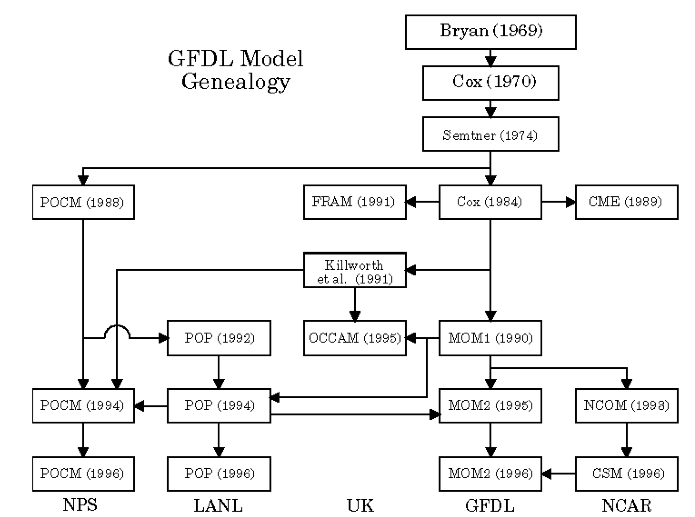
The Parallel Ocean Program (POP) was developed at LANL under the sponsorship of the Department of Energy’s CHAMMP program, which brought massively parallel computers to the realm of climate modeling. POP is a descendent of the Bryan-Cox-Semtner class of ocean models first developed by Kirk Bryan and Michael Cox [Bryan69] at the NOAA Geophysical Fluid Dynamics Laboratory in Princeton, NJ in the late 1960s. POP had its origins in a version of the model developed by Semtner and Chervin [Semtner86] [ChervinSemtner88]. The complete ‘’family tree’’ of the BCS models is displayed in the figure below (courtesy of Bert Semtner, Naval Postgraduate School).

Under the CHAMMP program, the Semtner-Chervin version was rewritten in CM Fortran for the Connection Machine CM-2 and CM-5 massively parallel computers. Experience with the resulting model led to a number of changes resulting in what is now known as the Parallel Ocean Program (POP). Although originally motivated by the adaptation of POP for massively parallel computers, many of these changes improved not only its computational performance but the fidelity of the model’s physical representation of the real ocean. The most significant of these improvements are summarized below. Details can be found in articles by Smith, [Smith et al 93], Dukowicz et al., [Dukowicz et al 93], and Dukowicz and Smith [Dukowicz and Smith94]. The model has continued to develop to adapt to new machines, incorporate new numerical algorithms and introduce new physical parameterizations.

1.2. Improvements introduced in POP

1.2.1. Surface-pressure formulation of barotropic mode

The barotropic streamfunction formulation in the standard BCS models required an additional equation to be solved for each continent and island that penetrated the ocean surface. This was costly even on machines like Cray parallel-vector-processor computers, which had fast memory access. To reduce the number of equations to solve with the barotropic streamfunction formulation, it was common practice to submerge islands, connect them to nearby continents with artificial land bridges, or merge an island chain into a single mass without gaps. The first modification created artificial gaps, permitting increased flow, while the latter two closed channels that should exist.

On distributed-memory parallel computers, these added equations were even more costly because each required gathering data from an arbitrarily large set of processors to perform a line-integral around each landmass. This computational dilemma was addressed by developing a new formulation of the barotropic mode based on surface pressure. The boundary condition for the surface pressure at a land-ocean interface point is local, which eliminates the non-local line-integral.

Consequently, the surface-pressure formulation permits any number of islands to be included at no additional computational cost, so all channels can be treated as precisely as the resolution of the grid permits.

Another problem with the barotropic streamfunction formulation is that the elliptic problem to be solved is ill-conditioned if bottom topography has large spatial gradients. The bottom topography must be smoothed to maintain numerical stability. Although this reduces the fidelity of the simulation, it does have the “desirable” side effect (given the other limitations of the streamfunction approach mentioned above) of submerging many islands, thereby reducing the number of equations to be solved. In contrast, the surface-pressure formulation allows more realistic, unsmoothed bottom topography to be used with no reduction in time step.

1.2.2. Free-surface boundary condition

The original ‘rigid-lid’ boundary condition was replaced by an implicit free-surface boundary condition that allows the air-sea interface to evolve freely and makes sea-surface height a prognostic variable.

1.2.3. Latitudinal scaling of horizontal diffusion

Scaling of the horizontal diffusion coefficient by was introduced, where θ is latitude, n = 1 for Laplacian mixing and n = 3 for bi-harmonic mixing. This optional scaling prevents horizontal diffusion from limiting the time step severely at high latitudes, yet keeps diffusion large enough to maintain numerical stability.

1.2.4. Pressure-averaging

After the temperature and salinity have been updated to time-step n + 1 in the baroclinic routines, the density and pressure can be computed. By computing the pressure gradient with a linear combination of at three time-levels , a technique well known in atmospheric modeling (BrownCampana[3]) it is possible to increase the time-step by as much as a factor of two.

1.2.5. Designed for parallel computers

The code is written in Fortran90 and can be run on a variety of parallel and serial computer architectures. Originally, the code was written using a data-parallel approach for the Thinking Machines Connection Machine. Later versions used a more traditional domain decomposition style using MPI or SHMEM for inter-processor communications. The most recent version of the code supports current clusters of shared-memory multi-processor nodes through the use of thread-based parallism (OpenMP) between processors on a node and message-passing (MPI or SHMEM) for communication between nodes. The flexibility of mixing thread-based and message-passing programming models gives the user the option of choosing the best combination of styles to suit a given machine.

1.2.6. General orthogonal coordinates in horizontal

The primitive equations were reformulated and discretized to allow the use of any locally orthogonal horizontal grid. This provides alternatives to the standard latitude-longitude grid with its singularity at the North Pole.

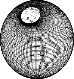
This generalization made possible the development of the displaced-pole grid, which moves the singularity arising from convergence of meridians at the North Pole into an adjacent landmass such as North America, Russia or Greenland. Such a displaced pole leaves a smooth, singularity-free grid in the Arctic Ocean. That grid joins smoothly at the equator with a standard Mercator grid in the Southern Hemisphere.

Note

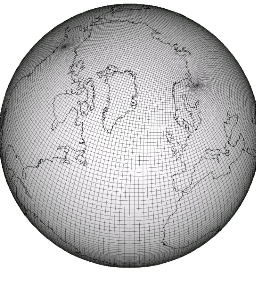
Supported grids in CESM1 include two displaced-pole grids, centered at Greenland, at nominal 1-degree (gx1v6) and 3-degree (gx3v7) horizontal resolution and 60 vertical levels. The most recent versions of the code also support a tripole grid in which two poles can be placed opposite each other in land masses near the North Pole to give more uniform grid spacing in the Arctic Ocean while maintaining all the advantages of the displaced pole grids.

Figure: Displaced-pole grid

POP2 also includes a high-resolution tripole grid at a nominal 0.1-degree horizontal resolution and 60 vertical levels. This grid is only supported technically: software-engineering tests at this resolution pass, i.e., there is presently only functional support for this grid.

Figure: Tripole grid

1.3. POP applications to date

1.3.1. High-resolution global and regional modeling

In the period 1994-97, POP was used to perform high resolution (0.28:sup:° at the Equator) global ocean simulations, running on the Thinking Machines CM5 computer then located at LANL’s Advanced Computing Laboratory. (Output from these runs is available at http://climate.acl.lanl.gov. The primary motivation for performing such high-resolution simulations is to resolve mesoscale eddies that play an important role in the dynamics of the ocean. Comparison of sea-surface height variability measured by the TOPEX/Poseidon satellite with that simulated by POP gave convincing evidence that still higher resolution was required (Fu and Smith[9]; Maltrud[15]).

At the time, it was not possible to do a higher resolution calculation on the global scale, so an Atlantic Ocean simulation was done with 0.1^° resolution at the Equator. This calculation agreed well with observations of sea-surface height variability in the Gulf Stream. Many other features of the flow were also well simulated (Smith et al [20]). Using the 0.1^° case as a benchmark, lower resolution cases were done at 0.2^° and 0.4^°; a comparison can be found at http://www.cgd.ucar.edu/oce/bryan/woce-poster.html.

Recently, it has become possible to begin a 0.1^° global simulation and such a simulation has been started. In addition, higher resolution North Atlantic simulations have also been initiated.

1.4. Running POP

POP requires some input data to run correctly. The first requirement is a file called *pop2\_in that contains many namelists that determine options and parameter values for the run. This input file will have been created by CIME for our case in the case $RUNDIR directory (and is also found in your $CASEROOT/CaseDocs directory as a reference.

In addition to pop2\_in, additional input files will be required to initialize grids, preconditioners, fields for output and possibly other options. These will be discussed in more detail in what follows.

The namelists and the model features that they control are presented in the following sections.

The namelists are presented in approximately the order in which they are called during the initialization of a POP run. However, some regrouping has been done to bring related topics together. The actual order of the namelists within the pop2\_in.file can be arbitrary; the code will search the file for the proper namelist to be read.

Todo

Put in link to the CIME guide to reference how namelists settings can be changed for pop and how POP is run as part of CIME - or simply duplicate that information here