CESM2-Large Ensemble Reproduction of Kay et al. 2015
Contents
CESM2-Large Ensemble Reproduction of Kay et al. 2015
Introduction
This Jupyter Notebook demonstrates how one might use the NCAR Community Earth System Model v2 (CESM2) Large Ensemble (CESM2-LE) data hosted on AWS S3. The notebook shows how to reproduce figure 2 from the Kay et al. (2015) paper describing the CESM LENS dataset (doi:10.1175/BAMS-D-13-00255.1), with the LENS2 dataset.
There was a previous notebook which explored this use case, put together by Joe Hamann and Anderson Banihirwe, accessible on the Pangeo Gallery using this link. The specific figure we are replicating is shown below.
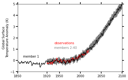
With the CESM2-LE dataset, we have 100 members which span from 1850 to 2100; whereas the original LENS dataset’s 40 member ensemble include data from 1920 to 2100. In this notebook, we include the ensemble spread from 1850 to 2100, comparing observations from the HADCRUT4 dataset when available. We also explore a more interactive version of this figure!
Imports
%matplotlib inline
import warnings

warnings.filterwarnings("ignore")

import intake
import numpy as np
import pandas as pd
import xarray as xr
import hvplot.pandas, hvplot.xarray
import holoviews as hv
from distributed import LocalCluster, Client
from ncar_jobqueue import NCARCluster
hv.extension('bokeh')


Spin up a Cluster
# If not using NCAR HPC, use the LocalCluster
#cluster = LocalCluster()
cluster = NCARCluster()
cluster.scale(40)

client = Client(cluster)
client
Client
Client-8d8f26fe-570c-11ec-8bf1-3cecef1b11fa
| Connection method: Cluster object | Cluster type: dask_jobqueue.PBSCluster |
| Dashboard: https://jupyterhub.hpc.ucar.edu/stable/user/mgrover/proxy/33398/status |
Cluster Info
PBSCluster
c44c2a68
| Dashboard: https://jupyterhub.hpc.ucar.edu/stable/user/mgrover/proxy/33398/status | Workers: 0 |
| Total threads: 0 | Total memory: 0 B |
Scheduler Info
Scheduler
Scheduler-e9ef908f-22e9-41fa-839d-795be56cd3d5
| Comm: tcp://10.12.206.54:46717 | Workers: 0 |
| Dashboard: https://jupyterhub.hpc.ucar.edu/stable/user/mgrover/proxy/33398/status | Total threads: 0 |
| Started: Just now | Total memory: 0 B |
Workers
Read in Data
Use the Intake-ESM Catalog to Access the Data
catalog = intake.open_esm_datastore(
    'https://raw.githubusercontent.com/NCAR/cesm2-le-aws/main/intake-catalogs/aws-cesm2-le.json'
)
catalog
aws-cesm2-le catalog with 34 dataset(s) from 318 asset(s):
| unique | |
|---|---|
| variable | 51 |
| long_name | 49 |
| component | 4 |
| experiment | 2 |
| forcing_variant | 2 |
| frequency | 3 |
| vertical_levels | 3 |
| spatial_domain | 3 |
| units | 20 |
| start_time | 4 |
| end_time | 7 |
| path | 297 |
Subset for Daily Temperature Data (TREFHT)
We use Intake-ESM here to query for our dataset, focusing the smoothed biomass burning (smbb) experiment!
catalog_subset = catalog.search(variable='TREFHT', frequency='daily')
catalog_subset
aws-cesm2-le catalog with 4 dataset(s) from 4 asset(s):
| unique | |
|---|---|
| variable | 1 |
| long_name | 1 |
| component | 1 |
| experiment | 2 |
| forcing_variant | 2 |
| frequency | 1 |
| vertical_levels | 1 |
| spatial_domain | 1 |
| units | 1 |
| start_time | 2 |
| end_time | 2 |
| path | 4 |
catalog_subset.df
| variable | long_name | component | experiment | forcing_variant | frequency | vertical_levels | spatial_domain | units | start_time | end_time | path | |
|---|---|---|---|---|---|---|---|---|---|---|---|---|
| 0 | TREFHT | reference height temperature | atm | historical | cmip6 | daily | 1.0 | global | K | 1850-01-01 12:00:00 | 2014-12-31 12:00:00 | s3://ncar-cesm2-lens/atm/daily/cesm2LE-histori... |
| 1 | TREFHT | reference height temperature | atm | historical | smbb | daily | 1.0 | global | K | 1850-01-01 12:00:00 | 2014-12-31 12:00:00 | s3://ncar-cesm2-lens/atm/daily/cesm2LE-histori... |
| 2 | TREFHT | reference height temperature | atm | ssp370 | cmip6 | daily | 1.0 | global | K | 2015-01-01 12:00:00 | 2100-12-31 12:00:00 | s3://ncar-cesm2-lens/atm/daily/cesm2LE-ssp370-... |
| 3 | TREFHT | reference height temperature | atm | ssp370 | smbb | daily | 1.0 | global | K | 2015-01-01 12:00:00 | 2100-12-31 12:00:00 | s3://ncar-cesm2-lens/atm/daily/cesm2LE-ssp370-... |
Taking a look at the dataframe, we see there are two files - one for the historical run, and the other a future scenario (ssp370)
catalog_subset.df
| variable | long_name | component | experiment | forcing_variant | frequency | vertical_levels | spatial_domain | units | start_time | end_time | path | |
|---|---|---|---|---|---|---|---|---|---|---|---|---|
| 0 | TREFHT | reference height temperature | atm | historical | cmip6 | daily | 1.0 | global | K | 1850-01-01 12:00:00 | 2014-12-31 12:00:00 | s3://ncar-cesm2-lens/atm/daily/cesm2LE-histori... |
| 1 | TREFHT | reference height temperature | atm | historical | smbb | daily | 1.0 | global | K | 1850-01-01 12:00:00 | 2014-12-31 12:00:00 | s3://ncar-cesm2-lens/atm/daily/cesm2LE-histori... |
| 2 | TREFHT | reference height temperature | atm | ssp370 | cmip6 | daily | 1.0 | global | K | 2015-01-01 12:00:00 | 2100-12-31 12:00:00 | s3://ncar-cesm2-lens/atm/daily/cesm2LE-ssp370-... |
| 3 | TREFHT | reference height temperature | atm | ssp370 | smbb | daily | 1.0 | global | K | 2015-01-01 12:00:00 | 2100-12-31 12:00:00 | s3://ncar-cesm2-lens/atm/daily/cesm2LE-ssp370-... |
Load in our datasets using .to_dataset_dict()
We use .to_dataset_dict() to return a dictionary of datasets, which we can now use for the analysis
dsets = catalog_subset.to_dataset_dict(storage_options={'anon':True})
--> The keys in the returned dictionary of datasets are constructed as follows:
	'component.experiment.frequency.forcing_variant'
Here are the keys for each dataset - you will notice they follow the groupby attributes, with component.experiment.frequency.forcing_variant, one for the future and the other historical here
dsets.keys()
dict_keys(['atm.historical.daily.smbb', 'atm.ssp370.daily.smbb', 'atm.historical.daily.cmip6', 'atm.ssp370.daily.cmip6'])
Let’s load these into separate datasets, then merge these together!
historical_smbb = dsets['atm.historical.daily.smbb']
future_smbb = dsets['atm.ssp370.daily.smbb']

historical_cmip6 = dsets['atm.historical.daily.cmip6']
future_cmip6 = dsets['atm.ssp370.daily.cmip6']
Now, we can merged the historical and future scenarios. We will drop any members that do not include the full 1850-2100 output!
merge_ds_smbb = xr.concat([historical_smbb, future_smbb], dim='time')
merge_ds_smbb = merge_ds_smbb.dropna(dim='member_id')

merge_ds_cmip6= xr.concat([historical_cmip6, future_cmip6], dim='time')
merge_ds_cmip6 = merge_ds_cmip6.dropna(dim='member_id')
For ease of plotting, we convert the cftime.datetime times to regular datetime
merge_ds_smbb['time'] = merge_ds_smbb.indexes['time'].to_datetimeindex()
merge_ds_cmip6['time'] = merge_ds_cmip6.indexes['time'].to_datetimeindex()
Finally, we can load in just the variable we are interested in, Reference height temperature (TREFHT). We will separate this into two arrays:
t_smbb- the entire period of data for the smoothed biomass burning experiment (1850 to 2100)t_cmip6- the entire period of data for the cmip6 biomass burning experiment (1850 to 2100)t_ref- the reference period used in the Kay et al. 2015 paper (1961 to 1990)
t_smbb = merge_ds_smbb.TREFHT
t_cmip6 = merge_ds_cmip6.TREFHT
t_ref = t_cmip6.sel(time=slice('1961', '1990'))
Read in the Grid Data
We also have Zarr stores of grid data, such as the area of each grid cell. We will need to follow a similar process here, querying for our experiment and extracting the dataset
grid_subset = catalog.search(component='atm', frequency='static', experiment='historical', forcing_variant='cmip6')
We can load in the dataset, calling pop_item, which grabs the dataset, assigning _ to the meaningless key
_, grid = grid_subset.to_dataset_dict(aggregate=False, zarr_kwargs={"consolidated": True}, storage_options={'anon':True}).popitem()
grid
--> The keys in the returned dictionary of datasets are constructed as follows:
	'variable.long_name.component.experiment.forcing_variant.frequency.vertical_levels.spatial_domain.units.start_time.end_time.path'
<xarray.Dataset>
Dimensions:   (lat: 192, lon: 288, ilev: 31, lev: 30, bnds: 2, slat: 191, slon: 288)
Coordinates: (12/21)
    P0        float64 ...
    area      (lat, lon) float32 dask.array<chunksize=(192, 288), meta=np.ndarray>
    gw        (lat) float64 dask.array<chunksize=(192,), meta=np.ndarray>
    hyai      (ilev) float64 dask.array<chunksize=(31,), meta=np.ndarray>
    hyam      (lev) float64 dask.array<chunksize=(30,), meta=np.ndarray>
    hybi      (ilev) float64 dask.array<chunksize=(31,), meta=np.ndarray>
    ...        ...
    ntrn      int32 ...
  * slat      (slat) float64 -89.53 -88.59 -87.64 -86.7 ... 87.64 88.59 89.53
  * slon      (slon) float64 -0.625 0.625 1.875 3.125 ... 355.6 356.9 358.1
    time      object ...
    w_stag    (slat) float64 dask.array<chunksize=(191,), meta=np.ndarray>
    wnummax   (lat) int32 dask.array<chunksize=(192,), meta=np.ndarray>
Dimensions without coordinates: bnds
Data variables:
    *empty*
Attributes:
    intake_esm_varname:      None
intake_esm_dataset_key: nan.nan.atm.historical.cmip6.static.nan.global.n...- lat: 192
- lon: 288
- ilev: 31
- lev: 30
- bnds: 2
- slat: 191
- slon: 288
- P0()float64...
- long_name :
- reference pressure
- units :
- Pa
array(nan)
- area(lat, lon)float32dask.array<chunksize=(192, 288), meta=np.ndarray>
- cell_methods :
- time: mean
- long_name :
- area of grid box
- units :
- m2
Array Chunk Bytes 216.00 kiB 216.00 kiB Shape (192, 288) (192, 288) Count 2 Tasks 1 Chunks Type float32 numpy.ndarray - gw(lat)float64dask.array<chunksize=(192,), meta=np.ndarray>
- long_name :
- gauss weights
Array Chunk Bytes 1.50 kiB 1.50 kiB Shape (192,) (192,) Count 2 Tasks 1 Chunks Type float64 numpy.ndarray - hyai(ilev)float64dask.array<chunksize=(31,), meta=np.ndarray>
- long_name :
- hybrid A coefficient at layer interfaces
Array Chunk Bytes 248 B 248 B Shape (31,) (31,) Count 2 Tasks 1 Chunks Type float64 numpy.ndarray - hyam(lev)float64dask.array<chunksize=(30,), meta=np.ndarray>
- long_name :
- hybrid A coefficient at layer midpoints
Array Chunk Bytes 240 B 240 B Shape (30,) (30,) Count 2 Tasks 1 Chunks Type float64 numpy.ndarray - hybi(ilev)float64dask.array<chunksize=(31,), meta=np.ndarray>
- long_name :
- hybrid B coefficient at layer interfaces
Array Chunk Bytes 248 B 248 B Shape (31,) (31,) Count 2 Tasks 1 Chunks Type float64 numpy.ndarray - hybm(lev)float64dask.array<chunksize=(30,), meta=np.ndarray>
- long_name :
- hybrid B coefficient at layer midpoints
Array Chunk Bytes 240 B 240 B Shape (30,) (30,) Count 2 Tasks 1 Chunks Type float64 numpy.ndarray - ilev(ilev)float642.255 5.032 10.16 ... 985.1 1e+03
- formula_terms :
- a: hyai b: hybi p0: P0 ps: PS
- long_name :
- hybrid level at interfaces (1000*(A+B))
- positive :
- down
- standard_name :
- atmosphere_hybrid_sigma_pressure_coordinate
- units :
- level
array([ 2.25524 , 5.031692, 10.157947, 18.555317, 30.669123, 45.867477, 63.323483, 80.701418, 94.941042, 111.693211, 131.401271, 154.586807, 181.863353, 213.952821, 251.704417, 296.117216, 348.366588, 409.835219, 482.149929, 567.224421, 652.332969, 730.445892, 796.363071, 845.353667, 873.715866, 900.324631, 924.964462, 947.432335, 967.538625, 985.11219 , 1000. ]) - lat(lat)float64-90.0 -89.06 -88.12 ... 89.06 90.0
- long_name :
- latitude
- units :
- degrees_north
array([-90. , -89.057592, -88.115183, -87.172775, -86.230366, -85.287958, -84.34555 , -83.403141, -82.460733, -81.518325, -80.575916, -79.633508, -78.691099, -77.748691, -76.806283, -75.863874, -74.921466, -73.979058, -73.036649, -72.094241, -71.151832, -70.209424, -69.267016, -68.324607, -67.382199, -66.439791, -65.497382, -64.554974, -63.612565, -62.670157, -61.727749, -60.78534 , -59.842932, -58.900524, -57.958115, -57.015707, -56.073298, -55.13089 , -54.188482, -53.246073, -52.303665, -51.361257, -50.418848, -49.47644 , -48.534031, -47.591623, -46.649215, -45.706806, -44.764398, -43.82199 , -42.879581, -41.937173, -40.994764, -40.052356, -39.109948, -38.167539, -37.225131, -36.282723, -35.340314, -34.397906, -33.455497, -32.513089, -31.570681, -30.628272, -29.685864, -28.743455, -27.801047, -26.858639, -25.91623 , -24.973822, -24.031414, -23.089005, -22.146597, -21.204188, -20.26178 , -19.319372, -18.376963, -17.434555, -16.492147, -15.549738, -14.60733 , -13.664921, -12.722513, -11.780105, -10.837696, -9.895288, -8.95288 , -8.010471, -7.068063, -6.125654, -5.183246, -4.240838, -3.298429, -2.356021, -1.413613, -0.471204, 0.471204, 1.413613, 2.356021, 3.298429, 4.240838, 5.183246, 6.125654, 7.068063, 8.010471, 8.95288 , 9.895288, 10.837696, 11.780105, 12.722513, 13.664921, 14.60733 , 15.549738, 16.492147, 17.434555, 18.376963, 19.319372, 20.26178 , 21.204188, 22.146597, 23.089005, 24.031414, 24.973822, 25.91623 , 26.858639, 27.801047, 28.743455, 29.685864, 30.628272, 31.570681, 32.513089, 33.455497, 34.397906, 35.340314, 36.282723, 37.225131, 38.167539, 39.109948, 40.052356, 40.994764, 41.937173, 42.879581, 43.82199 , 44.764398, 45.706806, 46.649215, 47.591623, 48.534031, 49.47644 , 50.418848, 51.361257, 52.303665, 53.246073, 54.188482, 55.13089 , 56.073298, 57.015707, 57.958115, 58.900524, 59.842932, 60.78534 , 61.727749, 62.670157, 63.612565, 64.554974, 65.497382, 66.439791, 67.382199, 68.324607, 69.267016, 70.209424, 71.151832, 72.094241, 73.036649, 73.979058, 74.921466, 75.863874, 76.806283, 77.748691, 78.691099, 79.633508, 80.575916, 81.518325, 82.460733, 83.403141, 84.34555 , 85.287958, 86.230366, 87.172775, 88.115183, 89.057592, 90. ]) - lat_bnds(lat, bnds)float64dask.array<chunksize=(192, 2), meta=np.ndarray>
Array Chunk Bytes 3.00 kiB 3.00 kiB Shape (192, 2) (192, 2) Count 2 Tasks 1 Chunks Type float64 numpy.ndarray - lev(lev)float643.643 7.595 14.36 ... 976.3 992.6
- formula_terms :
- a: hyam b: hybm p0: P0 ps: PS
- long_name :
- hybrid level at midpoints (1000*(A+B))
- positive :
- down
- standard_name :
- atmosphere_hybrid_sigma_pressure_coordinate
- units :
- level
array([ 3.643466, 7.59482 , 14.356632, 24.61222 , 38.2683 , 54.59548 , 72.012451, 87.82123 , 103.317127, 121.547241, 142.994039, 168.22508 , 197.908087, 232.828619, 273.910817, 322.241902, 379.100904, 445.992574, 524.687175, 609.778695, 691.38943 , 763.404481, 820.858369, 859.534767, 887.020249, 912.644547, 936.198398, 957.48548 , 976.325407, 992.556095]) - lon(lon)float640.0 1.25 2.5 ... 356.2 357.5 358.8
- long_name :
- longitude
- units :
- degrees_east
array([ 0. , 1.25, 2.5 , ..., 356.25, 357.5 , 358.75])
- lon_bnds(lon, bnds)float64dask.array<chunksize=(288, 2), meta=np.ndarray>
Array Chunk Bytes 4.50 kiB 4.50 kiB Shape (288, 2) (288, 2) Count 2 Tasks 1 Chunks Type float64 numpy.ndarray - ntrk()int32...
- long_name :
- spectral truncation parameter K
array(0, dtype=int32)
- ntrm()int32...
- long_name :
- spectral truncation parameter M
array(0, dtype=int32)
- ntrn()int32...
- long_name :
- spectral truncation parameter N
array(0, dtype=int32)
- slat(slat)float64-89.53 -88.59 ... 88.59 89.53
- long_name :
- staggered latitude
- units :
- degrees_north
array([-89.528796, -88.586387, -87.643979, -86.701571, -85.759162, -84.816754, -83.874346, -82.931937, -81.989529, -81.04712 , -80.104712, -79.162304, -78.219895, -77.277487, -76.335079, -75.39267 , -74.450262, -73.507853, -72.565445, -71.623037, -70.680628, -69.73822 , -68.795812, -67.853403, -66.910995, -65.968586, -65.026178, -64.08377 , -63.141361, -62.198953, -61.256545, -60.314136, -59.371728, -58.429319, -57.486911, -56.544503, -55.602094, -54.659686, -53.717277, -52.774869, -51.832461, -50.890052, -49.947644, -49.005236, -48.062827, -47.120419, -46.17801 , -45.235602, -44.293194, -43.350785, -42.408377, -41.465969, -40.52356 , -39.581152, -38.638743, -37.696335, -36.753927, -35.811518, -34.86911 , -33.926702, -32.984293, -32.041885, -31.099476, -30.157068, -29.21466 , -28.272251, -27.329843, -26.387435, -25.445026, -24.502618, -23.560209, -22.617801, -21.675393, -20.732984, -19.790576, -18.848168, -17.905759, -16.963351, -16.020942, -15.078534, -14.136126, -13.193717, -12.251309, -11.308901, -10.366492, -9.424084, -8.481675, -7.539267, -6.596859, -5.65445 , -4.712042, -3.769634, -2.827225, -1.884817, -0.942408, 0. , 0.942408, 1.884817, 2.827225, 3.769634, 4.712042, 5.65445 , 6.596859, 7.539267, 8.481675, 9.424084, 10.366492, 11.308901, 12.251309, 13.193717, 14.136126, 15.078534, 16.020942, 16.963351, 17.905759, 18.848168, 19.790576, 20.732984, 21.675393, 22.617801, 23.560209, 24.502618, 25.445026, 26.387435, 27.329843, 28.272251, 29.21466 , 30.157068, 31.099476, 32.041885, 32.984293, 33.926702, 34.86911 , 35.811518, 36.753927, 37.696335, 38.638743, 39.581152, 40.52356 , 41.465969, 42.408377, 43.350785, 44.293194, 45.235602, 46.17801 , 47.120419, 48.062827, 49.005236, 49.947644, 50.890052, 51.832461, 52.774869, 53.717277, 54.659686, 55.602094, 56.544503, 57.486911, 58.429319, 59.371728, 60.314136, 61.256545, 62.198953, 63.141361, 64.08377 , 65.026178, 65.968586, 66.910995, 67.853403, 68.795812, 69.73822 , 70.680628, 71.623037, 72.565445, 73.507853, 74.450262, 75.39267 , 76.335079, 77.277487, 78.219895, 79.162304, 80.104712, 81.04712 , 81.989529, 82.931937, 83.874346, 84.816754, 85.759162, 86.701571, 87.643979, 88.586387, 89.528796]) - slon(slon)float64-0.625 0.625 1.875 ... 356.9 358.1
- long_name :
- staggered longitude
- units :
- degrees_east
array([ -0.625, 0.625, 1.875, ..., 355.625, 356.875, 358.125])
- time()object...
- bounds :
- time_bnds
- long_name :
- time
array(cftime.DatetimeNoLeap(1850, 2, 1, 0, 0, 0, 0, has_year_zero=True), dtype=object) - w_stag(slat)float64dask.array<chunksize=(191,), meta=np.ndarray>
- long_name :
- staggered latitude weights
Array Chunk Bytes 1.49 kiB 1.49 kiB Shape (191,) (191,) Count 2 Tasks 1 Chunks Type float64 numpy.ndarray - wnummax(lat)int32dask.array<chunksize=(192,), meta=np.ndarray>
- long_name :
- cutoff Fourier wavenumber
Array Chunk Bytes 768 B 768 B Shape (192,) (192,) Count 2 Tasks 1 Chunks Type int32 numpy.ndarray
- intake_esm_varname :
- None
- intake_esm_dataset_key :
- nan.nan.atm.historical.cmip6.static.nan.global.nan.nan.nan.s3://ncar-cesm2-lens/atm/static/grid.zarr
Extract the Grid Area and Compute the Total Area
Here, we extract the grid area and compute the total area across all grid cells - this will help when computing the weights…
cell_area = grid.area.load()
total_area = cell_area.sum()
cell_area
<xarray.DataArray 'area' (lat: 192, lon: 288)>
array([[2.9948368e+07, 2.9948368e+07, 2.9948368e+07, ..., 2.9948368e+07,
        2.9948368e+07, 2.9948368e+07],
       [2.3957478e+08, 2.3957478e+08, 2.3957478e+08, ..., 2.3957478e+08,
        2.3957478e+08, 2.3957478e+08],
       [4.7908477e+08, 4.7908477e+08, 4.7908477e+08, ..., 4.7908477e+08,
        4.7908477e+08, 4.7908477e+08],
       ...,
       [4.7908477e+08, 4.7908477e+08, 4.7908477e+08, ..., 4.7908477e+08,
        4.7908477e+08, 4.7908477e+08],
       [2.3957478e+08, 2.3957478e+08, 2.3957478e+08, ..., 2.3957478e+08,
        2.3957478e+08, 2.3957478e+08],
       [2.9948368e+07, 2.9948368e+07, 2.9948368e+07, ..., 2.9948368e+07,
        2.9948368e+07, 2.9948368e+07]], dtype=float32)
Coordinates:
    P0       float64 nan
    area     (lat, lon) float32 2.995e+07 2.995e+07 ... 2.995e+07 2.995e+07
    gw       (lat) float64 nan nan nan nan nan nan ... nan nan nan nan nan nan
  * lat      (lat) float64 -90.0 -89.06 -88.12 -87.17 ... 87.17 88.12 89.06 90.0
  * lon      (lon) float64 0.0 1.25 2.5 3.75 5.0 ... 355.0 356.2 357.5 358.8
    ntrk     int32 0
    ntrm     int32 0
    ntrn     int32 0
    time     object 1850-02-01 00:00:00
    wnummax  (lat) int32 1543505128 10970 1543505128 ... 2146959360 0 2146959360
Attributes:
    cell_methods:  time: mean
    long_name:     area of grid box
units: m2- lat: 192
- lon: 288
- 2.995e+07 2.995e+07 2.995e+07 ... 2.995e+07 2.995e+07 2.995e+07
array([[2.9948368e+07, 2.9948368e+07, 2.9948368e+07, ..., 2.9948368e+07, 2.9948368e+07, 2.9948368e+07], [2.3957478e+08, 2.3957478e+08, 2.3957478e+08, ..., 2.3957478e+08, 2.3957478e+08, 2.3957478e+08], [4.7908477e+08, 4.7908477e+08, 4.7908477e+08, ..., 4.7908477e+08, 4.7908477e+08, 4.7908477e+08], ..., [4.7908477e+08, 4.7908477e+08, 4.7908477e+08, ..., 4.7908477e+08, 4.7908477e+08, 4.7908477e+08], [2.3957478e+08, 2.3957478e+08, 2.3957478e+08, ..., 2.3957478e+08, 2.3957478e+08, 2.3957478e+08], [2.9948368e+07, 2.9948368e+07, 2.9948368e+07, ..., 2.9948368e+07, 2.9948368e+07, 2.9948368e+07]], dtype=float32) - P0()float64nan
- long_name :
- reference pressure
- units :
- Pa
array(nan)
- area(lat, lon)float322.995e+07 2.995e+07 ... 2.995e+07
- cell_methods :
- time: mean
- long_name :
- area of grid box
- units :
- m2
array([[2.9948368e+07, 2.9948368e+07, 2.9948368e+07, ..., 2.9948368e+07, 2.9948368e+07, 2.9948368e+07], [2.3957478e+08, 2.3957478e+08, 2.3957478e+08, ..., 2.3957478e+08, 2.3957478e+08, 2.3957478e+08], [4.7908477e+08, 4.7908477e+08, 4.7908477e+08, ..., 4.7908477e+08, 4.7908477e+08, 4.7908477e+08], ..., [4.7908477e+08, 4.7908477e+08, 4.7908477e+08, ..., 4.7908477e+08, 4.7908477e+08, 4.7908477e+08], [2.3957478e+08, 2.3957478e+08, 2.3957478e+08, ..., 2.3957478e+08, 2.3957478e+08, 2.3957478e+08], [2.9948368e+07, 2.9948368e+07, 2.9948368e+07, ..., 2.9948368e+07, 2.9948368e+07, 2.9948368e+07]], dtype=float32) - gw(lat)float64nan nan nan nan ... nan nan nan nan
- long_name :
- gauss weights
array([nan, nan, nan, nan, nan, nan, nan, nan, nan, nan, nan, nan, nan, nan, nan, nan, nan, nan, nan, nan, nan, nan, nan, nan, nan, nan, nan, nan, nan, nan, nan, nan, nan, nan, nan, nan, nan, nan, nan, nan, nan, nan, nan, nan, nan, nan, nan, nan, nan, nan, nan, nan, nan, nan, nan, nan, nan, nan, nan, nan, nan, nan, nan, nan, nan, nan, nan, nan, nan, nan, nan, nan, nan, nan, nan, nan, nan, nan, nan, nan, nan, nan, nan, nan, nan, nan, nan, nan, nan, nan, nan, nan, nan, nan, nan, nan, nan, nan, nan, nan, nan, nan, nan, nan, nan, nan, nan, nan, nan, nan, nan, nan, nan, nan, nan, nan, nan, nan, nan, nan, nan, nan, nan, nan, nan, nan, nan, nan, nan, nan, nan, nan, nan, nan, nan, nan, nan, nan, nan, nan, nan, nan, nan, nan, nan, nan, nan, nan, nan, nan, nan, nan, nan, nan, nan, nan, nan, nan, nan, nan, nan, nan, nan, nan, nan, nan, nan, nan, nan, nan, nan, nan, nan, nan, nan, nan, nan, nan, nan, nan, nan, nan, nan, nan, nan, nan, nan, nan, nan, nan, nan, nan]) - lat(lat)float64-90.0 -89.06 -88.12 ... 89.06 90.0
- long_name :
- latitude
- units :
- degrees_north
array([-90. , -89.057592, -88.115183, -87.172775, -86.230366, -85.287958, -84.34555 , -83.403141, -82.460733, -81.518325, -80.575916, -79.633508, -78.691099, -77.748691, -76.806283, -75.863874, -74.921466, -73.979058, -73.036649, -72.094241, -71.151832, -70.209424, -69.267016, -68.324607, -67.382199, -66.439791, -65.497382, -64.554974, -63.612565, -62.670157, -61.727749, -60.78534 , -59.842932, -58.900524, -57.958115, -57.015707, -56.073298, -55.13089 , -54.188482, -53.246073, -52.303665, -51.361257, -50.418848, -49.47644 , -48.534031, -47.591623, -46.649215, -45.706806, -44.764398, -43.82199 , -42.879581, -41.937173, -40.994764, -40.052356, -39.109948, -38.167539, -37.225131, -36.282723, -35.340314, -34.397906, -33.455497, -32.513089, -31.570681, -30.628272, -29.685864, -28.743455, -27.801047, -26.858639, -25.91623 , -24.973822, -24.031414, -23.089005, -22.146597, -21.204188, -20.26178 , -19.319372, -18.376963, -17.434555, -16.492147, -15.549738, -14.60733 , -13.664921, -12.722513, -11.780105, -10.837696, -9.895288, -8.95288 , -8.010471, -7.068063, -6.125654, -5.183246, -4.240838, -3.298429, -2.356021, -1.413613, -0.471204, 0.471204, 1.413613, 2.356021, 3.298429, 4.240838, 5.183246, 6.125654, 7.068063, 8.010471, 8.95288 , 9.895288, 10.837696, 11.780105, 12.722513, 13.664921, 14.60733 , 15.549738, 16.492147, 17.434555, 18.376963, 19.319372, 20.26178 , 21.204188, 22.146597, 23.089005, 24.031414, 24.973822, 25.91623 , 26.858639, 27.801047, 28.743455, 29.685864, 30.628272, 31.570681, 32.513089, 33.455497, 34.397906, 35.340314, 36.282723, 37.225131, 38.167539, 39.109948, 40.052356, 40.994764, 41.937173, 42.879581, 43.82199 , 44.764398, 45.706806, 46.649215, 47.591623, 48.534031, 49.47644 , 50.418848, 51.361257, 52.303665, 53.246073, 54.188482, 55.13089 , 56.073298, 57.015707, 57.958115, 58.900524, 59.842932, 60.78534 , 61.727749, 62.670157, 63.612565, 64.554974, 65.497382, 66.439791, 67.382199, 68.324607, 69.267016, 70.209424, 71.151832, 72.094241, 73.036649, 73.979058, 74.921466, 75.863874, 76.806283, 77.748691, 78.691099, 79.633508, 80.575916, 81.518325, 82.460733, 83.403141, 84.34555 , 85.287958, 86.230366, 87.172775, 88.115183, 89.057592, 90. ]) - lon(lon)float640.0 1.25 2.5 ... 356.2 357.5 358.8
- long_name :
- longitude
- units :
- degrees_east
array([ 0. , 1.25, 2.5 , ..., 356.25, 357.5 , 358.75])
- ntrk()int320
- long_name :
- spectral truncation parameter K
array(0, dtype=int32)
- ntrm()int320
- long_name :
- spectral truncation parameter M
array(0, dtype=int32)
- ntrn()int320
- long_name :
- spectral truncation parameter N
array(0, dtype=int32)
- time()object1850-02-01 00:00:00
- bounds :
- time_bnds
- long_name :
- time
array(cftime.DatetimeNoLeap(1850, 2, 1, 0, 0, 0, 0, has_year_zero=True), dtype=object) - wnummax(lat)int321543505128 10970 ... 0 2146959360
- long_name :
- cutoff Fourier wavenumber
array([1543505128,      10970, 1543505128,      10970, 1543508400,
            10970, 1543508400,      10970,          0, 2146959360,
                0, 2146959360,          0, 2146959360,          0,
       2146959360,          0, 2146959360,          0, 2146959360,
                0, 2146959360,          0, 2146959360,          0,
       2146959360,          0, 2146959360,          0, 2146959360,
                0, 2146959360,          0, 2146959360,          0,
       2146959360,          0, 2146959360,          0, 2146959360,
                0, 2146959360,          0, 2146959360,          0,
       2146959360,          0, 2146959360,          0, 2146959360,
                0, 2146959360,          0, 2146959360,          0,
       2146959360,          0, 2146959360,          0, 2146959360,
                0, 2146959360,          0, 2146959360,          0,
       2146959360,          0, 2146959360,          0, 2146959360,
                0, 2146959360,          0, 2146959360,          0,
       2146959360,          0, 2146959360,          0, 2146959360,
                0, 2146959360,          0, 2146959360,          0,
       2146959360,          0, 2146959360,          0, 2146959360,
                0, 2146959360,          0, 2146959360,          0,
       2146959360,          0, 2146959360,          0, 2146959360,
                0, 2146959360,          0, 2146959360,          0,
       2146959360,          0, 2146959360,          0, 2146959360,
                0, 2146959360,          0, 2146959360,          0,
       2146959360,          0, 2146959360,          0, 2146959360,
                0, 2146959360,          0, 2146959360,          0,
       2146959360,          0, 2146959360,          0, 2146959360,
                0, 2146959360,          0, 2146959360,          0,
       2146959360,          0, 2146959360,          0, 2146959360,
                0, 2146959360,          0, 2146959360,          0,
       2146959360,          0, 2146959360,          0, 2146959360,
                0, 2146959360,          0, 2146959360,          0,
       2146959360,          0, 2146959360,          0, 2146959360,
                0, 2146959360,          0, 2146959360,          0,
       2146959360,          0, 2146959360,          0, 2146959360,
                0, 2146959360,          0, 2146959360,          0,
       2146959360,          0, 2146959360,          0, 2146959360,
                0, 2146959360,          0, 2146959360,          0,
       2146959360,          0, 2146959360,          0, 2146959360,
                0, 2146959360], dtype=int32)
- cell_methods :
- time: mean
- long_name :
- area of grid box
- units :
- m2
Compute the Weighted Annual Averages
Here, we utilize the resample(time="AS") method which does an annual resampling based on start of calendar year.
Note we also weight by the cell area, multiplying each value by the corresponding cell area, summing over the grid (lat, lon), then dividing by the total area
Setup the Computation - Below, we lazily prepare the calculation!
You’ll notice how quickly this cell runs - which is suspicious 👀 - we didn’t actually do any computation, but rather prepared the calculation
%%time
t_ref_ts = (
    (t_ref.resample(time="AS").mean("time")).weighted(cell_area).mean(('lat', 'lon'))
).mean(dim=("time", "member_id"))

t_smbb_ts = (
    (t_smbb.resample(time="AS").mean("time")).weighted(cell_area).mean(('lat', 'lon')))

t_cmip6_ts = (
    (t_cmip6.resample(time="AS").mean("time")).weighted(cell_area).mean(('lat', 'lon')))
CPU times: user 1.63 s, sys: 20.7 ms, total: 1.65 s
Wall time: 1.74 s
Compute the Averages
At this point, we actually compute the averages - using %%time to help us measure how long it takes to compute…
%%time
t_ref_mean = t_ref_ts.compute()
CPU times: user 17.5 s, sys: 552 ms, total: 18 s
Wall time: 41.4 s
%%time
t_smbb_mean = t_smbb_ts.compute()
CPU times: user 1min 37s, sys: 3.41 s, total: 1min 41s
Wall time: 3min 14s
%%time
t_cmip6_mean = t_cmip6_ts.compute()
CPU times: user 2min 32s, sys: 4.84 s, total: 2min 37s
Wall time: 5min 36s
Convert to Dataframes
Our output data format is still an xarray.DataArray which isn’t neccessarily ideal… we could convert this to a dataframe which would be easier to export.
For example, you could call anomaly_smbb.to_csv('some_output_file.csv') to export to csv, which you could then share with others!
We can convert our xarray.DataArray to a pandas dataframe using the following:
t_smbb_ts_df = t_smbb_mean.to_series().unstack().T
t_cmip6_ts_df = t_cmip6_mean.to_series().unstack().T
Now that we have our dataframes, we can compute the anomaly by subtracting the mean value t_ref_mean
anomaly_smbb = (t_smbb_ts_df - t_ref_mean.data)
anomaly_cmip6 = (t_cmip6_ts_df - t_ref_mean.data)
Grab some Observational Data
In this case, we use the HADCRUT4 dataset. We include the url here, which can be used to remotely access the data.
# Observational time series data for comparison with ensemble average
obsDataURL = "https://www.esrl.noaa.gov/psd/thredds/dodsC/Datasets/cru/hadcrut4/air.mon.anom.median.nc"
ds = xr.open_dataset(obsDataURL).load()
ds
<xarray.Dataset>
Dimensions:    (lat: 36, lon: 72, time: 2061, nbnds: 2)
Coordinates:
  * lat        (lat) float32 87.5 82.5 77.5 72.5 ... -72.5 -77.5 -82.5 -87.5
  * lon        (lon) float32 -177.5 -172.5 -167.5 -162.5 ... 167.5 172.5 177.5
  * time       (time) datetime64[ns] 1850-01-01 1850-02-01 ... 2021-09-01
Dimensions without coordinates: nbnds
Data variables:
    time_bnds  (time, nbnds) datetime64[ns] 1850-01-01 1850-01-31 ... 2021-09-30
    air        (time, lat, lon) float32 nan nan nan nan nan ... nan nan nan nan
Attributes:
    platform:                        Surface
    title:                           HADCRUT4 Combined Air Temperature/SST An...
    history:                         Originally created at NOAA/ESRL PSD by C...
    Conventions:                     CF-1.0
    Comment:                         This dataset supersedes V3
    Source:                          Obtained from http://hadobs.metoffice.co...
    version:                         4.2.0
    dataset_title:                   HadCRUT4
    References:                      https://www.psl.noaa.gov/data/gridded/da...
DODS_EXTRA.Unlimited_Dimension: time- lat: 36
- lon: 72
- time: 2061
- nbnds: 2
- lat(lat)float3287.5 82.5 77.5 ... -82.5 -87.5
- long_name :
- Latitude
- units :
- degrees_north
- actual_range :
- [ 87.5 -87.5]
- axis :
- Y
- coordinate_defines :
- point
- standard_name :
- latitude
- _ChunkSizes :
- 36
array([ 87.5, 82.5, 77.5, 72.5, 67.5, 62.5, 57.5, 52.5, 47.5, 42.5, 37.5, 32.5, 27.5, 22.5, 17.5, 12.5, 7.5, 2.5, -2.5, -7.5, -12.5, -17.5, -22.5, -27.5, -32.5, -37.5, -42.5, -47.5, -52.5, -57.5, -62.5, -67.5, -72.5, -77.5, -82.5, -87.5], dtype=float32) - lon(lon)float32-177.5 -172.5 ... 172.5 177.5
- long_name :
- Longitude
- units :
- degrees_east
- actual_range :
- [-177.5 177.5]
- axis :
- X
- coordinate_defines :
- point
- standard_name :
- longitude
- _ChunkSizes :
- 72
array([-177.5, -172.5, -167.5, -162.5, -157.5, -152.5, -147.5, -142.5, -137.5, -132.5, -127.5, -122.5, -117.5, -112.5, -107.5, -102.5, -97.5, -92.5, -87.5, -82.5, -77.5, -72.5, -67.5, -62.5, -57.5, -52.5, -47.5, -42.5, -37.5, -32.5, -27.5, -22.5, -17.5, -12.5, -7.5, -2.5, 2.5, 7.5, 12.5, 17.5, 22.5, 27.5, 32.5, 37.5, 42.5, 47.5, 52.5, 57.5, 62.5, 67.5, 72.5, 77.5, 82.5, 87.5, 92.5, 97.5, 102.5, 107.5, 112.5, 117.5, 122.5, 127.5, 132.5, 137.5, 142.5, 147.5, 152.5, 157.5, 162.5, 167.5, 172.5, 177.5], dtype=float32) - time(time)datetime64[ns]1850-01-01 ... 2021-09-01
- long_name :
- Time
- delta_t :
- 0000-01-00 00:00:00
- avg_period :
- 0000-01-00 00:00:00
- standard_name :
- time
- axis :
- T
- coordinate_defines :
- start
- bounds :
- time_bnds
- actual_range :
- [18262. 80962.]
- _ChunkSizes :
- 1
array(['1850-01-01T00:00:00.000000000', '1850-02-01T00:00:00.000000000',
       '1850-03-01T00:00:00.000000000', ..., '2021-07-01T00:00:00.000000000',
       '2021-08-01T00:00:00.000000000', '2021-09-01T00:00:00.000000000'],
      dtype='datetime64[ns]')
- time_bnds(time, nbnds)datetime64[ns]1850-01-01 ... 2021-09-30
- long_name :
- Time Boundaries
- _ChunkSizes :
- [1 2]
array([['1850-01-01T00:00:00.000000000', '1850-01-31T00:00:00.000000000'], ['1850-02-01T00:00:00.000000000', '1850-02-28T00:00:00.000000000'], ['1850-03-01T00:00:00.000000000', '1850-03-31T00:00:00.000000000'], ..., ['2021-07-01T00:00:00.000000000', '2021-07-31T00:00:00.000000000'], ['2021-08-01T00:00:00.000000000', '2021-08-31T00:00:00.000000000'], ['2021-09-01T00:00:00.000000000', '2021-09-30T00:00:00.000000000']], dtype='datetime64[ns]') - air(time, lat, lon)float32nan nan nan nan ... nan nan nan nan
- dataset :
- HADCRUT4
- var_desc :
- Air Temperature
- level_desc :
- Surface
- statistic :
- Anomaly
- parent_stat :
- Observation
- valid_range :
- [-40. 40.]
- units :
- degC
- long_name :
- HADCRUT4: Median Surface Air Temperature Monthly Median Anomaly from 100 ensemble members
- precision :
- 2
- cell_methods :
- time: anomaly (monthly from values)
- standard_name :
- air_temperature_anomaly
- actual_range :
- [-9.9692100e+36 2.0620308e+01]
- _ChunkSizes :
- [ 1 36 72]
array([[[        nan,         nan,         nan, ...,         nan,
                 nan,         nan],
        [        nan,         nan,         nan, ...,         nan,
                 nan,         nan],
        [        nan,         nan,         nan, ...,         nan,
                 nan,         nan],
        ...,
        [        nan,         nan,         nan, ...,         nan,
                 nan,         nan],
        [        nan,         nan,         nan, ...,         nan,
                 nan,         nan],
        [        nan,         nan,         nan, ...,         nan,
                 nan,         nan]],

       [[        nan,         nan,         nan, ...,         nan,
                 nan,         nan],
        [        nan,         nan,         nan, ...,         nan,
                 nan,         nan],
        [        nan,         nan,         nan, ...,         nan,
                 nan,         nan],
...
        [        nan,         nan,         nan, ..., -2.7343245 ,
                 nan,         nan],
        [        nan,         nan,         nan, ...,         nan,
                 nan,         nan],
        [        nan,         nan,         nan, ...,         nan,
                 nan,         nan]],

       [[        nan,         nan,         nan, ...,         nan,
                 nan,         nan],
        [        nan,  0.07189226,  0.29999995, ...,         nan,
                 nan,         nan],
        [        nan,         nan,  0.2679553 , ...,         nan,
                 nan,         nan],
        ...,
        [        nan,         nan,         nan, ...,  3.3641    ,
                 nan,         nan],
        [        nan,         nan,         nan, ...,         nan,
                 nan,         nan],
        [        nan,         nan,         nan, ...,         nan,
                 nan,         nan]]], dtype=float32)
- platform :
- Surface
- title :
- HADCRUT4 Combined Air Temperature/SST Anomaly
- history :
- Originally created at NOAA/ESRL PSD by CAS 04/2012 from files obtained at the Hadley Center
- Conventions :
- CF-1.0
- Comment :
- This dataset supersedes V3
- Source :
- Obtained from http://hadobs.metoffice.com/ Data is a collaboration of CRU and the Hadley Center
- version :
- 4.2.0
- dataset_title :
- HadCRUT4
- References :
- https://www.psl.noaa.gov/data/gridded/data.hadcrut4.html
- DODS_EXTRA.Unlimited_Dimension :
- time
Compute the Weighted Temporal Mean from Seasons
This observational dataset comes in as seasonal values, but we want yearly averages.. this requires weighting by the length of each season, so we include this helper function, weighted_temporal_mean!
def weighted_temporal_mean(ds):
    """
    weight by days in each month
    """
    time_bound_diff = ds.time_bnds.diff(dim="nbnds")[:, 0]
    wgts = time_bound_diff.groupby("time.year") / time_bound_diff.groupby(
        "time.year"
    ).sum(xr.ALL_DIMS)
    np.testing.assert_allclose(wgts.groupby("time.year").sum(xr.ALL_DIMS), 1.0)
    obs = ds["air"]
    cond = obs.isnull()
    ones = xr.where(cond, 0.0, 1.0)
    obs_sum = (obs * wgts).resample(time="AS").sum(dim="time")
    ones_out = (ones * wgts).resample(time="AS").sum(dim="time")
    obs_s = (obs_sum / ones_out).mean(("lat", "lon")).to_series()
    return obs_s
Let’s apply this to our dataset now!
obs_s = weighted_temporal_mean(ds)
obs_s
time
1850-01-01   -0.338822
1851-01-01   -0.245482
1852-01-01   -0.291014
1853-01-01   -0.342457
1854-01-01   -0.276820
                ...
2017-01-01    0.777498
2018-01-01    0.641953
2019-01-01    0.809306
2020-01-01    0.865248
2021-01-01    0.677946
Freq: AS-JAN, Length: 172, dtype: float64
Convert the dataset into a dataframe
obs_df = pd.DataFrame(obs_s).rename(columns={0:'value'})
obs_df
| value | |
|---|---|
| time | |
| 1850-01-01 | -0.338822 |
| 1851-01-01 | -0.245482 |
| 1852-01-01 | -0.291014 |
| 1853-01-01 | -0.342457 |
| 1854-01-01 | -0.276820 |
| ... | ... |
| 2017-01-01 | 0.777498 |
| 2018-01-01 | 0.641953 |
| 2019-01-01 | 0.809306 |
| 2020-01-01 | 0.865248 |
| 2021-01-01 | 0.677946 |
172 rows × 1 columns
Plot the Output
In this this case, we use hvPlot to plot the output! We setup the plots in the following cell
smbb_plot = (
    anomaly_smbb.hvplot.scatter(
        'time',
        height=300,
        width=500,
        color='lightgrey',
        legend=False,
        xlabel='Year',
        ylabel='Global Mean \n Temperature Anomaly (K)',
        ylim=(-1, 5),
        hover=False,
    )
    * anomaly_smbb.mean(1).hvplot.line('time', color='k', line_width=3, label='ensemble mean')
    * obs_df.hvplot.line('time', color='red', label='observations')
).opts(title='Smoothed Biomass Burning')


cmip6_plot = (
    anomaly_cmip6.hvplot.scatter(
        'time',
        height=300,
        width=500,
        color='lightgrey',
        legend=False,
        xlabel='Year',
        ylabel='Global Mean \n Temperature Anomaly (K)',
        ylim=(-1, 5),
        hover=False,
    )
    * anomaly_cmip6.mean(1).hvplot.line('time', color='k', line_width=3, label='ensemble mean')
    * obs_df.hvplot.line('time', color='red', label='observations').opts(
        title='CMIP6 Biomass Burning'
    )
)

# Include both plots in the same column
(smbb_plot + cmip6_plot).cols(1)
Spin Down the Cluster
After we are done, we can spin down our cluster
cluster.close()
client.close()