Frequently Asked Questions#

This page contains answers to frequently asked questions from the ESDS Zulip and office hours.

Help topics:#

Where do I go for help?

What do I do if my question is not answered on this page?

Someone must have written the function I want. Where do I look?

How do I use conda environments?

Xarray and Dask

GitHub

CESM Data

Where do I go for help?#

Try one of the following resources.

Xarray’s How Do I do X? page
Xarray Github Discussions
Pangeo Discourse Forum
ESDS Zulip under #python-questions, #python-dev, or #dask.

Avoid personal emails and prefer a public forum.

What do I do if my question is not answered on this page?#

If your question is related to conda environments and you’re affiliated with NSF NCAR or UCAR, you can open a help ticket on the NSF NCAR Research Computing Helpdesk site. If your issue is related to data science packages and workflows, you can open an issue on our GitHub repository here or book an office hours appointment with an ESDS core member!

Someone must have written the function I want. Where do I look?#

See the xarray related projects page. Also see the xarray-contrib and pangeo-data GitHub organizations. Some NSF NCAR relevant projects include:

How do I use conda environments?#

General Advice#

Dealing with Python environments can be tricky… a good place to start is to checkout this guide to dealing with Python environments.

If you just need a refresher on the various conda commands, this conda cheet sheet is a wonderful quick reference.

Using conda on NSF NCAR HPC resources#

Warning

Since 12 December 2022, it is no longer recommended to install your own version of miniconda on the HPC system. To export your existing environments to the recommended installation of miniconda, refer to the “How can I export my environments?” section.

The NSF NCAR High Performance Computing (HPC) systems have a conda installation for you to use. The most recent and detailed instructions can be found on this Using Conda and Python page.

If you don’t want the trouble of making your own conda environment, there are managed environments available. The NSF NCAR Package Library (NPL) is an environment containing many common scientific Python pacakges such as Numpy, Xarray, and GeoCAT. You can access the NPL environment through the command line and the NSF NCAR JupyterHub.

NPL on the command line#

Open up a terminal on Casper or Derecho
Load the conda module:
```
$ module load conda
```
List the available managed environments:
```
$ conda env list
```
Activate the environment you want to use. Here we are using the npl environment as an example. npl can be replaced with any available environment name:
```
$ conda activate npl
```
Now when you run a script, the modules within the npl environment will be available to your program.

NPL on the NSF NCAR JupyterHub#

Log in to the Production NSF NCAR JupyterHub
Start a server
With your Jupyter Notebook open, click on the kernel name in the upper right.
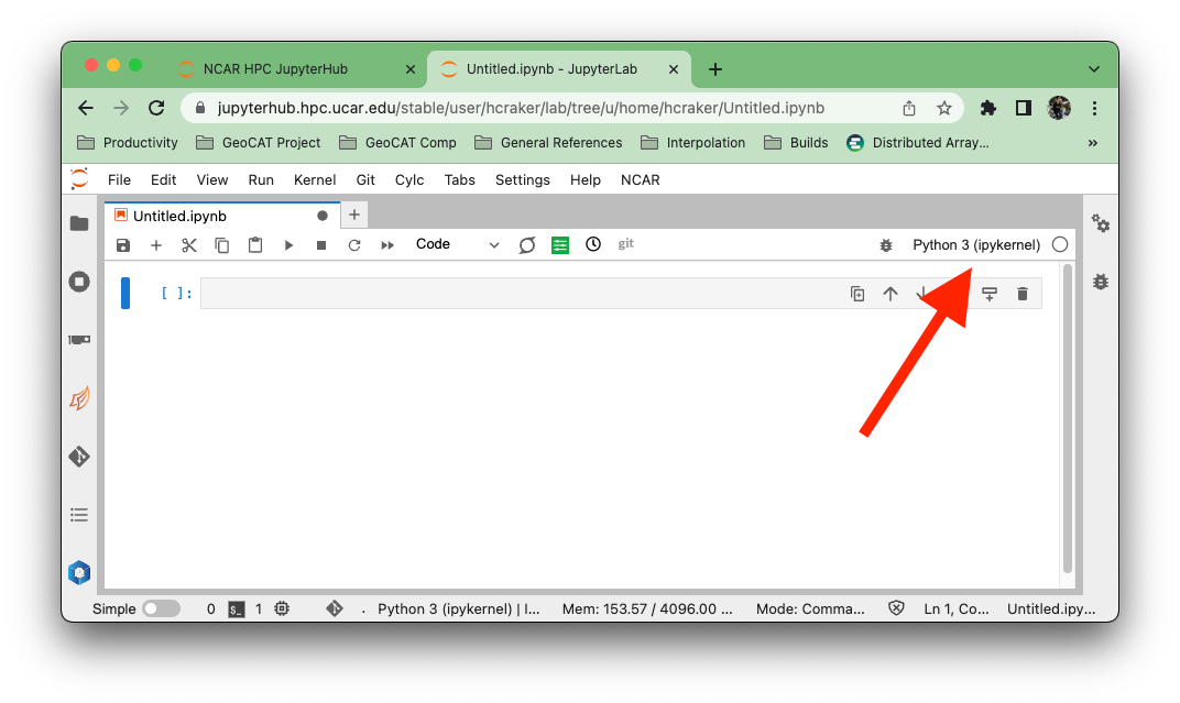
A dialog will appear with all the verious kernels available to you. These kernels will (generally) have the same name as the conda environment that it uses. This may not be the case if you are managing your own environments and kernels.
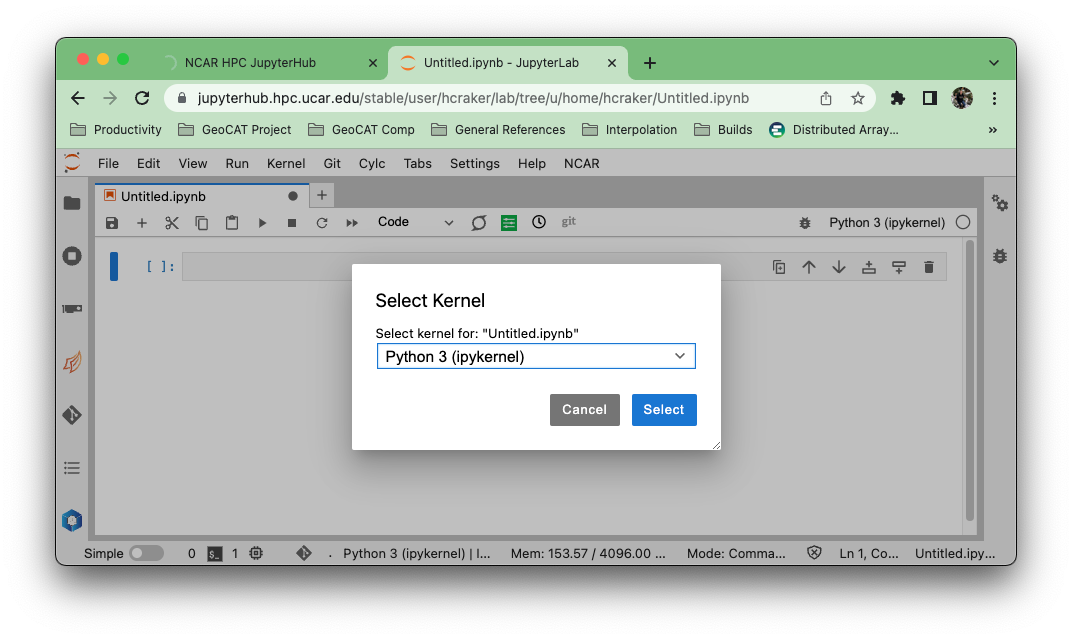
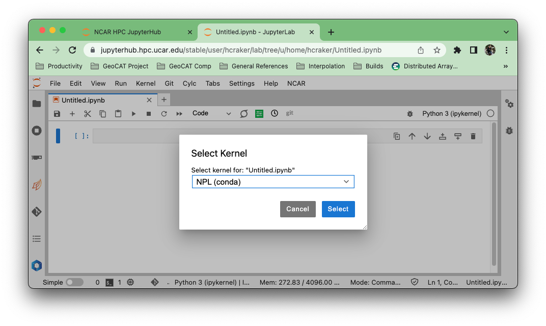
Select the “npl (conda)” kernel from the list if you want to use the NSF NCAR-managed NPL environment.

Creating and accessing a new conda environment on the NSF NCAR JupyterHub#

You may want to move past using NPL, and create a new conda environment! For detailed instructions, check out the Using Conda and Python page on the NSF NCAR Advanced Research Computing site. Heres a summary of the basic steps:

Create the environment

If you are creating an environment from scratch, use the following:
```
conda create --name my_environment
```
where my_environment is the name of your environment

Ff you have an environment file (ex. environment.yml), use the following:
```
conda env create -f environment.yml
```
Activate your environment and install the ipykernel package
```
conda activate my_environment.yml
conda install ipykernel
```
Note

The ipykernel package is required for your environment to be available from the NSF NCAR JupyterHub
Accessing your conda environment

Your environment should now automatically show up as an available kernel in any Jupyter server on the NSF NCAR HPC systems. If you want to give your kernel a name that is different from the environment name, you can use the following command:
```
python -m ipykernel install --user --name=my-kernel
```
Where my-kernel is the kernel name.

Conda is taking too long to solve environment: use mamba#

This is a very common issue when installing a new package or trying to update a package in an existing conda environment. This issue is usually manifested in a conda message along these lines:

environment Solving environment: failed with initial frozen solve. Retrying with flexible solve.

One solution to this issue is to use mamba which is a drop-in replacement for conda. Mamba aims to greately speed up and improve conda functionality such as solving environment, installing packages, etc…

Installing Mamba

conda install -n base -c conda-forge mamba

Set conda-forge and nodefaults channels

conda config --add channels nodefaults
conda config --add channels conda-forge

To install a package with mamba, you just run

mamba install package_name

To create/update an environment from an environment file, run:

mamba env update -f environment.yml

Note

We do not recommend using mamba to activate and deactivate environments as this can cause packages to misbehave/not load correctly.

See mamba documentation for more.

How can I export my environments?#

If you made an environment on one machine or using a different conda installation, you can export that environment and use it elsewhere. These are the basic steps:

Export your environment

With the environment you want to export activated, run the following command:
```
conda env export --from-history > environment.yml
```
where environment can be replaced with the file name of your choice. The --from-history flag allows you to recreate your environment on any system. It is the cross-platform compatible way of exporting an environment.
Move the environment.yml to the system you want to use it on / activate the appropriate conda installtion you wish to use.
Use the .yml file to create your environment
```
conda env create -f environment.yml
```

Xarray and Dask#

General tips#

Read the xarray documentation on optimizing workflow with dask.
Read the Best practices for Dask array
Keep track of chunk sizes throughout your workflow. This is especially important when reading in data using xr.open_mfdataset. Aim for 100-200MB size chunks.
Choose chunking appropriate to your analysis. If you’re working with time series, then chunk more in space and less along time.
Avoid indexing with .where as much as possible. In particulate .where(..., drop=True) will trigger a compute since it needs to know where NaNs are present to drop them. Instead see if you can write your statement as a .clip, .sel, .isel, or .query statement.

How do I optimize reading multiple files using Xarray and Dask?#

A good first place to start when reading in multiple files is Xarray’s multi-file documentation.

For example, if you are trying to read in multiple files where you are interested in concatenating over the time dimension, here is an example of the xr.open_dataset line would look like:

ds = xr.open_mfdataset(
        files,
        # Name of the dimension to concatenate along.
        concat_dim="time",

        # Attempt to auto-magically combine the given datasets into one by using dimension coordinates.
        combine="by_coords",

        # Specify chunks for dask - explained later
        chunks={"lev": 1, "time": 500},

        # Only data variables in which the dimension already appears are included.
        data_vars="minimal",

        # Only coordinates in which the dimension already appears are included.
        coords="minimal",

        # Skip comparing and pick variable from first dataset.
        compat="override",
        parallel=True,
    )

Where can I find Xarray tutorials?#

See videos and notebooks.

How do I debug my code when using Dask?#

An option is to use .compute(scheduler="single-threaded"). This will run your code as a serial for loop. When an error is raised you can use the %debug magic to drop in to the stack and debug from there. See this post for more debugging tips in a serial context.

`KilledWorker` X{. What do I do?#

Keep an eye on the dask dashboard.

If a lot of the bars in the Memory tab are orange, that means your workers are running out of memory. Reduce your chunk size.

Help, my analysis is slow!#

Try subsetting for just the variable(s) you need for example, if you are reading in a dataset with ~25 variables, and you only need temperature, just read in temperature. You can specificy which variables to read in by using the following syntax, following the example of the temperature variable.

ds = xr.open_dataset(file, data_vars=['temperature'])

Take a look at your chunk size, it might not be optimized. When reading a file in using Xarray with Dask, a “general rule of thumb” is to keep your chunk size down to around 100 mb.

For example, let’s say you trying to read in multiple files, each with ~600 time steps. This is case where each file is very large (several 10s of GB) and using Dask to help with data processing is essential.

You can check the size of each chunk by subsetting a single DataArray (ex. ds['temperature'])

If you have very large chunks, try modifying the number of chunks you specify within xr.open_mfdataset(files, ..., chunks={'lev':1, "time": 500}) where lev and time are vertical and time dimensions respectively.

Check to see how large each chunk is after modifying the chunk size, and modify as necessary.

You do not have enough dask workers

If you have a few large files, having the number of workers equal to to the number of input files read in using xr.open_mfdataset would be a good practice

If you have a large number of smaller files, you may not run into this issue, and it is suggest you look at the other potential solutions.

I have to do lots of rechunking, but the rechunk step uses too much memory and kills my workers.#

Try the rechunker package.

Writing to files in parallel#

Distributed writes to netCDF are hard.

Try writing to zarr using Dataset.to_zarr.
If you need to write to netCDF and your final dataset can fit in memory then use dataset.load().to_netcdf(...).
If you really must write a big dataset to netCDF try using save_mfdataset (see here).

My Dask workers are taking a long time to start. How can I monitor them?#

Dask worker requests are added to the job queues on Casper and Derecho with the cluster.scale() method. After this method is called, you can verify that they are waiting in the queue with this command:

qstat -u <my_username> on Derecho, and the same command will work on Casper after April 2021.

If you see no pending worker jobs, then verify that you have called cluster.scale().

GitHub#

Setting up GitHub Authentication#

Beginning August 13, 2021, GitHub will no longer accept account passwords when authenticating git operations. There are essentially two options, which GitHub provides proper documentation for getting setup:

CESM Data#

Dealing with CESM monthly output - is there something wrong with time#

A well known issue of CESM data is that timestamps for fields saved as averages are placed at the end of the averaging period. For instance, in the following example, the January/1920 average has a timestamp of February/1920:

In [25]: filename = '/glade/collections/cdg/data/cesmLE/CESM-CAM5-BGC-LE/atm/proc/tseries/monthly/TS/b.e11.B20TRC5CNBDRD.f09_g16.011.cam.h0.TS.192001-200512.nc'

In [33]: ds = xr.open_dataset(filename)

In [34]: ds.time
Out[34]:
<xarray.DataArray 'time' (time: 1032)>
array([cftime.DatetimeNoLeap(1920, 2, 1, 0, 0, 0, 0),
       cftime.DatetimeNoLeap(1920, 3, 1, 0, 0, 0, 0),
       cftime.DatetimeNoLeap(1920, 4, 1, 0, 0, 0, 0), ...,
       cftime.DatetimeNoLeap(2005, 11, 1, 0, 0, 0, 0),
       cftime.DatetimeNoLeap(2005, 12, 1, 0, 0, 0, 0),
       cftime.DatetimeNoLeap(2006, 1, 1, 0, 0, 0, 0)], dtype=object)
Coordinates:
  * time     (time) object 1920-02-01 00:00:00 ... 2006-01-01 00:00:00
Attributes:
    long_name:  time
    bounds:     time_bnds

A temporary workaround is to fix the issue ourselves by computing new time axis by averaging the time bounds:

In [29]: import xarray as xr

In [30]: import cf_xarray # use cf-xarray so that we can use CF attributes

In [31]: filename = '/glade/collections/cdg/data/cesmLE/CESM-CAM5-BGC-LE/atm/proc/tseries/monthly/TS/b.e11.B20TRC5CNBDRD.f09_g16.011.cam.h0.TS.192001-200512.nc'

In [32]: ds = xr.open_dataset(filename)

In [34]: attrs, encoding = ds.time.attrs.copy(), ds.time.encoding.copy()

In [36]: time_bounds = ds.cf.get_bounds('time')

In [37]: time_bounds_dim_name = ds.cf.get_bounds_dim_name('time')

In [38]: ds = ds.assign_coords(time=time_bounds.mean(time_bounds_dim_name))

In [39]: ds.time.attrs, ds.time.encoding = attrs, encoding

In [40]: ds.time
Out[40]:
<xarray.DataArray 'time' (time: 1032)>
array([cftime.DatetimeNoLeap(1920, 1, 16, 12, 0, 0, 0),
       cftime.DatetimeNoLeap(1920, 2, 15, 0, 0, 0, 0),
       cftime.DatetimeNoLeap(1920, 3, 16, 12, 0, 0, 0), ...,
       cftime.DatetimeNoLeap(2005, 10, 16, 12, 0, 0, 0),
       cftime.DatetimeNoLeap(2005, 11, 16, 0, 0, 0, 0),
       cftime.DatetimeNoLeap(2005, 12, 16, 12, 0, 0, 0)], dtype=object)
Coordinates:
  * time     (time) object 1920-01-16 12:00:00 ... 2005-12-16 12:00:00
Attributes:
    long_name:  time
    bounds:     time_bnds