Annual Maximum JJA Heat Index at Boulder, CO and Chicago, IL (1990–2025)
ERA5 and JRA-3Q Reanalyses from NCAR GDEX
Scientific motivation
This notebook computes the annual maximum June–July–August (JJA) heat index at two mid-latitude United States cities — Boulder, Colorado (semi-arid, elevation 1655 m) and Chicago, Illinois (humid continental, Lake Michigan influence) — using two independent global reanalyses spanning 1990–2025.
The analysis follows the methodology of Romps (2024), who demonstrated using ERA5 that the annual maximum summer heat index in Texas has increased at a rate several times larger than the contemporaneous increase in dry-bulb temperature. The physical basis for this amplification lies in the nonlinearity of the heat index with respect to temperature and humidity: at near-saturated conditions, the Clausius–Clapeyron relation implies that a given increment of warming produces a disproportionately large increase in physiological heat stress. Chicago, situated in a persistently humid air mass, is expected to exhibit stronger amplification than semi-arid Boulder, where the heat index remains close to the dry-bulb temperature throughout the summer.
Datasets
| Product | GDEX identifier | Temporal resolution | Quantity archived | Access format |
|---|---|---|---|---|
| ERA5 surface analysis | d633000 | Hourly instantaneous | VAR_2T, VAR_2D | Native Zarr |
JRA-3Q surface analysis (anl_surf125) | d640000 | 6-hourly instantaneous | TMP_GDS0_HTGL, RH_GDS0_HTGL | kerchunk reference |
Because ERA5 provides 24 candidate values per day versus 4 for JRA-3Q, computing the JJA season maximum from the full hourly ERA5 stream would systematically inflate ERA5 relative to JRA-3Q through a sample-size effect alone. To remove this artifact, ERA5 is subsampled to one randomly selected observation per 6-hour window prior to computing the annual maximum, matching the JRA-3Q cadence. A random draw, rather than a fixed synoptic hour, is used to avoid introducing a systematic diurnal-phase bias into the sampled ERA5 distribution. We re-sample instead of taking a mean over a 6-hour window because the average might miss an extreme heat index value in this window.
Heat index formulation
The heat index is computed using the heatindex Python package of Lu & Romps
(2025), which implements the extended formulation of Lu & Romps (2022) in python.
The function takes air temperature in Kelvin and relative humidity on the
interval and returns the heat index in Kelvin:
hi.heatindex(T_K, rh) → HI_KERA5 does not archive near-surface relative humidity directly. It is derived from
the 2-m temperature (VAR_2T) and 2-m dew-point temperature (VAR_2D) via the
August–Roche–Magnus approximation, consistent with the ECMWF IFS documentation.
JRA-3Q provides relative humidity in percent as RH_GDS0_HTGL in the surface
analysis product.
Required Packages
Please make sure to install the packages before moving forward
intake
intake-esm >= 2025.12.12
xarray
dask
zarr
kerchunk
numpy
pandas
matplotlib
heatindex >= 0.0.2
!pip install heatindexDefaulting to user installation because normal site-packages is not writeable
Requirement already satisfied: heatindex in /glade/u/home/harshah/.local/lib/python3.10/site-packages (0.0.2)
Requirement already satisfied: numpy in /glade/u/home/harshah/.local/lib/python3.10/site-packages (from heatindex) (1.26.4)
[notice] A new release of pip is available: 25.3 -> 26.0.1
[notice] To update, run: pip install --upgrade pip
import matplotlib.pyplot as plt
import numpy as np
import os
import xarray as xr
import intake
import intake_esm
import pandas as pd
import cartopy.crs as ccrs
import cartopy.feature as cfeature
import dask
from dask_jobqueue import PBSCluster
from dask.distributed import Client
Step 1 - Locate the Dataset
On the NCAR GDEX portal, go to the Data Access tab for the ERA5/ JRA-3Q dataset to find the intake-ESM catalogs needed to access data. In this notebook we will use GDEX POSIX catalog.
# Please specify your preferred data access method: the Data URL or the GDEX POSIX path.
era5_catalog_posix = '/gdex/data/d633000/catalogs/d633000-posix.json'
jra3q_catalog_posix = '/gdex/data/d640000/catalogs/d640000-posix.json'
Step 2 - Set up cluster
# Set up your sratch folder path
username       = os.environ["USER"]
glade_scratch  = "/glade/derecho/scratch/" + username
print(glade_scratch)
/glade/derecho/scratch/harshah
# Create a PBS cluster object
cluster = PBSCluster(
    job_name = 'dask-wk25',
    cores = 1,
    memory = '8GiB',
    processes = 1,
    local_directory = glade_scratch+'/dask/spill/',
    log_directory = glade_scratch + '/dask/logs/',
    resource_spec = 'select=1:ncpus=1:mem=8GB',
    queue = 'casper',
    walltime = '5:00:00',
    interface = 'ext'
)

# Create the client to load the Dashboard
client = Client(cluster)

n_workers = 5
cluster.scale(n_workers)
client.wait_for_workers(n_workers = n_workers)
cluster
/glade/u/home/harshah/venvs/mdm/lib/python3.10/site-packages/distributed/node.py:187: UserWarning: Port 8787 is already in use.
Perhaps you already have a cluster running?
Hosting the HTTP server on port 45117 instead
warnings.warn(
Step 3 - Open the catalog, find and load the variable of interest
%%time
era5_cat = intake.open_esm_datastore(era5_catalog_posix)
jra3q_cat = intake.open_esm_datastore(jra3q_catalog_posix)
era5_cat
CPU times: user 9.97 ms, sys: 301 μs, total: 10.3 ms
Wall time: 9.73 ms
# ── Time range ────────────────────────────────────────────────────────────────
YEAR_START_ERA5  = 1990
YEAR_START_JRA3Q = 1990
YEAR_END         = 2025

JJA_MONTHS = [6, 7, 8]

# ── Site coordinates (degrees north, degrees east 0–360) ──────────────────────
SITES = {
    "Boulder_CO" : {"lat":  40.01, "lon": 254.73},
    "Chicago_IL" : {"lat":  41.88, "lon": 272.37},
}

# ── Reproducibility ───────────────────────────────────────────────────────────
RANDOM_SEED = 42

# ── Output ────────────────────────────────────────────────────────────────────
OUTPUT_ZARR = glade_scratch + "/max_jja_ehi_boulder_chicago.zarr"
Search for humidity and temperature variables in the catalog using the long_name and/or short_name columns. We only show the JRA-3Q example in the code below
jra3q_cat.df[['variable', 'short_name', 'long_name']].drop_duplicates().loc[
jra3q_cat.df['long_name'].str.contains('2m temp|humid', case=False, na=False)]# ERA5: 2-m temperature and 2-m dew-point (GDEX convention)
ERA5_T_VAR = "VAR_2T"
ERA5_TD_VAR = "VAR_2D"
era5_search = era5_cat.search(variable=[ERA5_T_VAR, ERA5_TD_VAR])
print(f"ERA5 matched: {len(era5_search.df):,} entries")
# JRA-3Q: 2-m temperature and 2-m relative humidity
# Variable names confirmed from the discovery step in the previous cell:
# tmp2m-hgt-an-ll125 → 2-metre temperature, height level, analysis
# rh2m-hgt-an-ll125 → 2-metre relative humidity, height level, analysis
JRA3Q_T_VAR = "tmp2m-hgt-an-ll125"
JRA3Q_RH_VAR = "rh2m-hgt-an-ll125"
jra3q_search = jra3q_cat.search(variable=[JRA3Q_T_VAR, JRA3Q_RH_VAR])
print(f"JRA-3Q matched: {len(jra3q_search.df):,} entries")ERA5 matched: 2 entries
JRA-3Q matched: 2 entries
Now that we have figured out the correct variable names, let us load the data using xarray
#Use paths to the load the dataset
era5_t_path  = era5_search.df.loc[era5_search.df['variable'] == ERA5_T_VAR,  'path'].item()
era5_td_path = era5_search.df.loc[era5_search.df['variable'] == ERA5_TD_VAR, 'path'].item()

jra3q_t_path  = jra3q_search.df.loc[jra3q_search.df['variable'] == JRA3Q_T_VAR,  'path'].item()
jra3q_rh_path = jra3q_search.df.loc[jra3q_search.df['variable'] == JRA3Q_RH_VAR, 'path'].item()

# print(era5_t_path)
# print(era5_td_path)
# print(jra3q_t_path)
# print(jra3q_rh_path)
%%time
era5_t_ds = xr.open_zarr(era5_t_path, chunks={})[[ERA5_T_VAR]]
era5_td_ds = xr.open_zarr(era5_td_path, chunks={})[[ERA5_TD_VAR]]
era5_ds = xr.merge([era5_t_ds, era5_td_ds])
#
era5_dsCPU times: user 383 ms, sys: 113 ms, total: 497 ms
Wall time: 542 ms
jra3q_ds   = xr.open_dataset(jra3q_t_path, engine='kerchunk', chunks={})[[JRA3Q_T_VAR, JRA3Q_RH_VAR]]
jra3q_dsExtract data
Resample ERA5 data to 6hr frequency
Subset the data in space (Colorado and Chicago) and time
# Subset to analysis period and JJA
era5_ds  = era5_ds.sel(time=slice(str(YEAR_START_ERA5),  str(YEAR_END)))
jra3q_ds = jra3q_ds.sel(time=slice(str(YEAR_START_JRA3Q), str(YEAR_END)))

era5_ds  = era5_ds.sel(time=era5_ds.time.dt.month.isin(JJA_MONTHS))
jra3q_ds = jra3q_ds.sel(time=jra3q_ds.time.dt.month.isin(JJA_MONTHS))

#
# Extract nearest grid cell for each site
era5_points  = {}
jra3q_points = {}

for site, coords in SITES.items():
    lat, lon = coords["lat"], coords["lon"]

    era5_pt  = era5_ds.sel(latitude=lat, longitude=lon, method="nearest")
    jra3q_pt = jra3q_ds.sel(lat=lat,     lon=lon,       method="nearest")

    print(f"ERA5   / {site}: requested ({lat:.2f}°N, {lon:.2f}°E) → "
          f"nearest ({float(era5_pt.latitude):.3f}°N, {float(era5_pt.longitude):.3f}°E)")
    print(f"JRA-3Q / {site}: requested ({lat:.2f}°N, {lon:.2f}°E) → "
          f"nearest ({float(jra3q_pt.lat):.3f}°N, {float(jra3q_pt.lon):.3f}°E)")

    era5_points[site]  = era5_pt
    jra3q_points[site] = jra3q_pt
ERA5 / Boulder_CO: requested (40.01°N, 254.73°E) → nearest (40.000°N, 254.750°E)
JRA-3Q / Boulder_CO: requested (40.01°N, 254.73°E) → nearest (40.000°N, 255.000°E)
ERA5 / Chicago_IL: requested (41.88°N, 272.37°E) → nearest (42.000°N, 272.250°E)
JRA-3Q / Chicago_IL: requested (41.88°N, 272.37°E) → nearest (42.500°N, 272.500°E)
# Randomly subsample ERA5 to one observation per 6-hour window
# to match the JRA-3Q temporal cadence prior to computing the annual maximum

def subsample_6h_random(ds, seed=RANDOM_SEED):
    """
    Retain one randomly selected observation per 6-hour window.
    The selection mask is built from the time coordinate only,
    leaving data variables Dask-lazy.
    """
    times        = pd.DatetimeIndex(ds["time"].values)
    window_start = times.floor("6h")
    unique_wins  = np.unique(window_start)

    rng           = np.random.default_rng(seed)
    offsets_h     = rng.integers(0, 6, size=len(unique_wins)).astype(int)
    win_to_offset = dict(zip(unique_wins, offsets_h))

    pos_h = ((times - window_start).total_seconds() / 3600).astype(int)
    keep  = np.fromiter(
        (pos_h[i] == win_to_offset[window_start[i]] for i in range(len(times))),
        dtype=bool,
        count=len(times),
    )

    print(f"  {ds.sizes['time']:,} → {keep.sum():,} time steps retained "
          f"({keep.sum() / len(times) * 100:.1f}%, expected ≈16.7%)")
    return ds.isel(time=keep)


for site in SITES:
    era5_points[site] = subsample_6h_random(era5_points[site])
    print(f"ERA5 / {site}: subsampling complete")
78,000 → 13,000 time steps retained (16.7%, expected ≈16.7%)
ERA5 / Boulder_CO: subsampling complete
78,000 → 13,000 time steps retained (16.7%, expected ≈16.7%)
ERA5 / Chicago_IL: subsampling complete
# Derive relative humidity from ERA5 2-m temperature and dew-point temperature.
# Following Romps (2024, supplementary section 1.5), relative humidity is computed
# as the ratio of the saturation vapor pressure evaluated at the dew-point temperature
# to that evaluated at the air temperature. The saturation vapor pressure is
# approximated using the August-Roche-Magnus formula (Alduchov and Eskridge, 1996).
#
# Alduchov, O.A. and Eskridge, R.E., 1996. Improved Magnus form approximation of
# saturation vapor pressure. Journal of Applied Meteorology and Climatology, 35(4),
# pp.601-609. DOI: 10.1175/1520-0450(1996)035<0601:IMFAOS>2.0.CO;2
#
# JRA-3Q provides relative humidity directly in %; convert to [0, 1].

def rh_from_T_Td(T_K, Td_K):
    a, b = 17.625, 243.04
    T_C  = T_K  - 273.15
    Td_C = Td_K - 273.15
    rh   = np.exp(a * Td_C / (b + Td_C)) / np.exp(a * T_C  / (b + T_C))
    return rh.clip(0.0, 1.0)


for site in SITES:
    era5_points[site] = era5_points[site].assign(
        rh=rh_from_T_Td(era5_points[site][ERA5_T_VAR],era5_points[site][ERA5_TD_VAR]))

    jra3q_points[site] = jra3q_points[site].assign(rh=(jra3q_points[site][JRA3Q_RH_VAR] / 100.0).clip(0.0, 1.0))

print("Relative humidity prepared for all sites.")
Relative humidity prepared for all sites.
Step 4 - Data Analysis
%%time
from heatindex import heatindex

def compute_heatindex_xr(T_K, rh):
    """
    Compute the extended heat index (Lu and Romps, 2022) using the
    Python implementation of Romps (2024).

    Parameters
    ----------
    T_K : xr.DataArray  — 2-m temperature in Kelvin
    rh  : xr.DataArray  — relative humidity in [0, 1]

    Returns
    -------
    xr.DataArray — heat index in Kelvin
    """
    hi_K = xr.apply_ufunc(
        heatindex,
        T_K,
        rh,
        dask="parallelized",
        output_dtypes=[float],
    )
    hi_K.attrs = {"units": "K", "long_name": "Heat Index (Lu and Romps, 2022)"}
    return hi_K


# Compute heat index and annual maximum JJA value for each site
results = {}

for site in SITES:
    results[site] = {}
    for label, points in [("ERA5", era5_points), ("JRA-3Q", jra3q_points)]:
        ds   = points[site]
        T_K  = ds[ERA5_T_VAR]  if label == "ERA5" else ds[JRA3Q_T_VAR]
        rh   = ds["rh"]

        hi_K     = compute_heatindex_xr(T_K, rh)
        ann_max  = hi_K.groupby("time.year").max(dim="time")

        print(f"Computing {label} / {site} ...")
        results[site][label] = (ann_max - 273.15).compute()
        print(f"  Done. Years: {int(results[site][label].year[0])}–"
              f"{int(results[site][label].year[-1])}")
Computing ERA5 / Boulder_CO ...
Done. Years: 1990–2025
Computing JRA-3Q / Boulder_CO ...
/glade/u/home/harshah/venvs/mdm/lib/python3.10/site-packages/distributed/client.py:3383: UserWarning: Sending large graph of size 28.14 MiB.
This may cause some slowdown.
Consider loading the data with Dask directly
 or using futures or delayed objects to embed the data into the graph without repetition.
See also https://docs.dask.org/en/stable/best-practices.html#load-data-with-dask for more information.
  warnings.warn(
  Done. Years: 1990–2025
Computing ERA5 / Chicago_IL ...
  Done. Years: 1990–2025
Computing JRA-3Q / Chicago_IL ...
/glade/u/home/harshah/venvs/mdm/lib/python3.10/site-packages/distributed/client.py:3383: UserWarning: Sending large graph of size 28.24 MiB.
This may cause some slowdown.
Consider loading the data with Dask directly
 or using futures or delayed objects to embed the data into the graph without repetition.
See also https://docs.dask.org/en/stable/best-practices.html#load-data-with-dask for more information.
  warnings.warn(
Done. Years: 1990–2025
out_vars = {}

for site in SITES:
    slug = site.lower()
    for label, da in results[site].items():
        key = f"{label.lower().replace('-', '')}_{slug}_hi_max_jja"
        da  = da.drop_vars(["latitude", "longitude", "lat", "lon"], errors="ignore")
        da  = da.rename(key)
        out_vars[key] = da

ds_out = xr.Dataset(out_vars)
ds_out.to_zarr(OUTPUT_ZARR, mode="w")
print(f"Results written to: {OUTPUT_ZARR}")
print(xr.open_zarr(OUTPUT_ZARR))
Results written to: /glade/derecho/scratch/harshah/max_jja_ehi_boulder_chicago.zarr
<xarray.Dataset> Size: 1kB
Dimensions: (year: 36)
Coordinates:
* year (year) int64 288B 1990 1991 1992 ... 2024 2025
Data variables:
era5_boulder_co_hi_max_jja (year) float64 288B dask.array<chunksize=(36,), meta=np.ndarray>
era5_chicago_il_hi_max_jja (year) float64 288B dask.array<chunksize=(36,), meta=np.ndarray>
jra3q_boulder_co_hi_max_jja (year) float64 288B dask.array<chunksize=(36,), meta=np.ndarray>
jra3q_chicago_il_hi_max_jja (year) float64 288B dask.array<chunksize=(36,), meta=np.ndarray>
%%time
fig, ax = plt.subplots(figsize=(10, 5))

colors = {"Boulder_CO": "tab:blue", "Chicago_IL": "tab:red"}
ls     = {"ERA5": "-", "JRA-3Q": "--"}

for site in SITES:
    for label, da in results[site].items():
        ax.plot(
            da.year,
            da.values,
            color     = colors[site],
            linestyle = ls[label],
            linewidth = 1.5,
            label     = f"{site.replace('_', ', ')} — {label}",
        )

ax.set_xlabel("Year")
ax.set_ylabel("Annual maximum JJA heat index (°C)")
ax.set_title("Annual Maximum JJA Heat Index\nBoulder, CO and Chicago, IL (1990–2025)")
ax.legend(framealpha=0.9)
ax.grid(linestyle=":", alpha=0.5)
plt.tight_layout()
plt.show()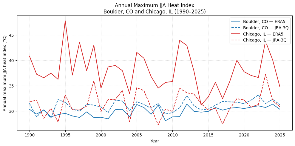
CPU times: user 184 ms, sys: 47.1 ms, total: 231 ms
Wall time: 258 ms
The plot confirms our intuition: Chicago, a more humid place, has a higher JJA maximum heat index than Boulder
We see the infamous 1995 Chicago Heat Wave in the plot, but it is not captured by JRA-3Q!
For both Chicago and Boulder, the predictions from both the ERA5 and JRA-3Q reanalyses seem to broadly agree!
# Close the cluster
cluster.close()
References
Romps, D.M., 2024. Heat index extremes increasing several times faster than the air temperature, ERL, 2024 Environmental Research Letters
Lu, Y.-C. and Romps, D.M., 2022. Extending the heat index. Journal of Applied Meteorology and Climatology, 61(10), 1367–1383. DOI: Lu & Romps (2022)
Lu, Y.-C. and Romps, D.M., 2025.
heatindex: Tools for Calculating Heat Stress, version 0.0.2. https://heatindex .org Hersbach, H., et al., 2020. The ERA5 global reanalysis. Quarterly Journal of the Royal Meteorological Society, 146(730), 1999–2049. DOI: Hersbach et al. (2020)
Kosaka, Y., et al., 2024. The JRA-3Q Reanalysis. Journal of the Meteorological Society of Japan, 102, 49–109. DOI: KOSAKA et al. (2024)
- Lu, Y.-C., & Romps, D. M. (2022). Extending the Heat Index. Journal of Applied Meteorology and Climatology, 61(10), 1367–1383. 10.1175/jamc-d-22-0021.1
- Hersbach, H., Bell, B., Berrisford, P., Hirahara, S., Horányi, A., Muñoz‐Sabater, J., Nicolas, J., Peubey, C., Radu, R., Schepers, D., Simmons, A., Soci, C., Abdalla, S., Abellan, X., Balsamo, G., Bechtold, P., Biavati, G., Bidlot, J., Bonavita, M., … Thépaut, J. (2020). The ERA5 global reanalysis. Quarterly Journal of the Royal Meteorological Society, 146(730), 1999–2049. 10.1002/qj.3803
- KOSAKA, Y., KOBAYASHI, S., HARADA, Y., KOBAYASHI, C., NAOE, H., YOSHIMOTO, K., HARADA, M., GOTO, N., CHIBA, J., MIYAOKA, K., SEKIGUCHI, R., DEUSHI, M., KAMAHORI, H., NAKAEGAWA, T., TANAKA, T. Y., TOKUHIRO, T., SATO, Y., MATSUSHITA, Y., & ONOGI, K. (2024). The JRA-3Q Reanalysis. Journal of the Meteorological Society of Japan. Ser. II, 102(1), 49–109. 10.2151/jmsj.2024-004