Access [DATASET-NAME] through the NCAR GDEX
Required Packages
Here we will list the required packages (try only include the necessary packages for this example) to be able to perform the following steps. Please make sure to installed the packages before moving forward
package1...
Step 1 - Define the Simple Research Question
Lorem ipsum dolor sit amet, consectetur adipiscing elit. Sed do eiusmod tempor incididunt ut labore et dolore magna aliqua. Ut enim ad minim veniam, quis nostrud exercitation ullamco laboris nisi ut aliquip ex ea commodo consequat. Duis aute irure dolor in reprehenderit in voluptate velit esse cillum dolore eu fugiat nulla pariatur. Excepteur sint occaecat cupidatat non proident, sunt in culpa qui officia deserunt mollit anim id est laborum.
Step 2 - Locate the Dataset
On the NCAR GDEX portal, go to the Data Access tab for your selected dataset.... A text description is enough but feel free to include print screen or movies if it helps. Please specify your preferred data access method: the Data URL or the GDEX POSIX path. We are also open to suggestions for the most useful access method for our target users.
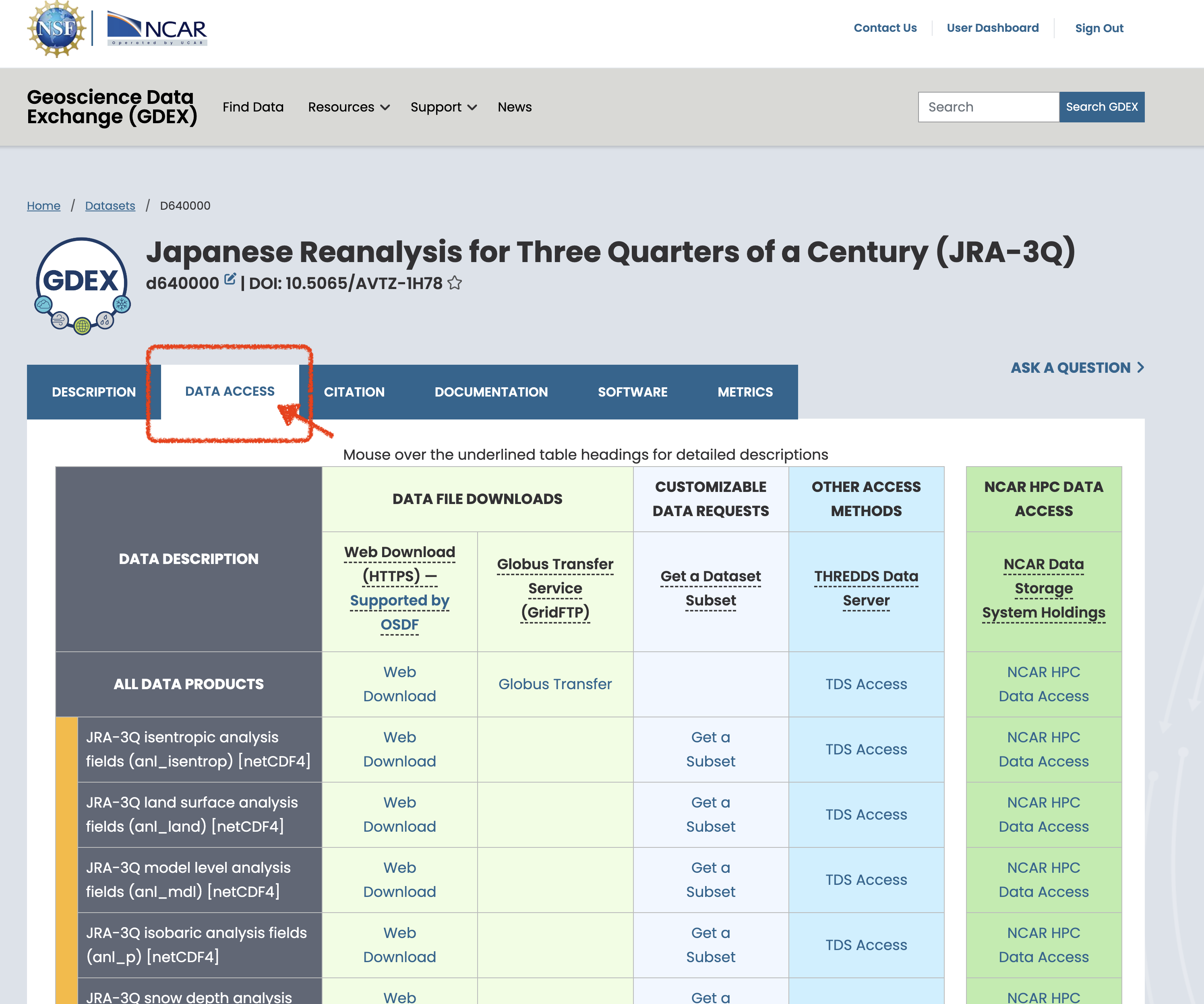
Figure 1:Steps to Find the Data! Any movie or png files can be put in ../docs/images/ with specific names to the file.
# Please specify your preferred data access method: the Data URL or the GDEX POSIX path.
# We are also open to suggestions for the most useful access method for our target users.
data_url = "https://data.gdex.ucar.edu/d640000/catalogs/d640000-https.json"
data_posix_path = "/gdex/data/d640000/catalogs/d640000-https.json"
Step 3 - Open the Data
This is the steps to show how to load or lazy load the data into the current notebook
import xarray as xr
ds = xr.open_dataset(data_url)
ds = xr.open_dataset(data_posix_path)
Step 4 - Focus on the Variable addressing the Research Question
A quick filtering through various filtering, preprocessing or slicing can be shown here
Step 5 - Data Analysis
The research focus analysis can be shown below. A plotted figures from time to time will usually be benefitial to understand the various analysis steps.
# a quick one time slice glance of the data
ds['tmp2m-hgt-an-gauss'].isel(time=0).plot(cmap='coolwarm')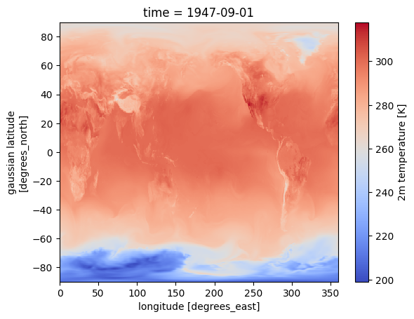
%%time
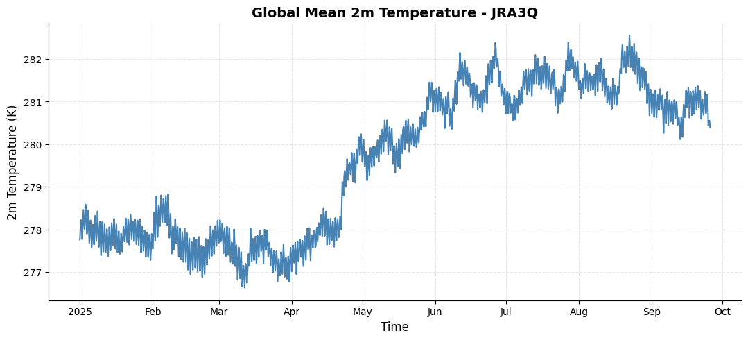
# a quick calculation of global mean surface temperature hourly time series
da_tmp2m = ds['tmp2m-hgt-an-gauss'].sel(time=slice('2025-01-01','2025-09-25')).mean(dim=['lat','lon']).compute()
CPU times: user 2min 22s, sys: 2.21 s, total: 2min 25s
Wall time: 2min
import matplotlib.pyplot as plt

# Create a customized time series plot
fig = plt.figure(figsize=(10, 4))
ax = fig.add_axes([0, 0, 1, 1])

# plot time series
da_tmp2m.plot(ax=ax, color='steelblue', linewidth=1.5)

# Customize the plot
ax.set_title('Global Mean 2m Temperature - JRA3Q', fontsize=14, fontweight='bold')
ax.set_xlabel('Time', fontsize=12)
ax.set_ylabel('2m Temperature (K)', fontsize=12)
ax.grid(True, alpha=0.3, linestyle='--')
ax.spines['top'].set_visible(False)
ax.spines['right'].set_visible(False)