Working with Curly Vectors

Overview

Ultraplot

Ultraplot is a wrapper for Matplotlib. Curly vectors can be created via the curved_quiver()

import numpy as np
import matplotlib.pyplot as plt
import ultraplot as uplot

# Sample data
x = np.linspace(-3, 3, 30)
y = np.linspace(-3, 3, 30)
X, Y = np.meshgrid(x, y)
v = X  # the y-component
u = -Y  # the x-component

# plot
fig, ax = uplot.subplot(figsize=(8, 8))

ax.curved_quiver(
    x=X,
    y=Y,
    u=u,
    v=v,
    color="red",
    arrow_at_end=True,
    arrowsize=1,
    linewidth=1,
    density=10,
)

ax.format(suptitle='UltraPlot - Curly Vector Plot', grid=True, xlabel='x', ylabel='y')

plt.show()

/home/runner/micromamba/envs/geocat-applications/lib/python3.14/site-packages/ultraplot/__init__.py:227: UltraPlotWarning: Rebuilding font cache. This usually happens after installing or updating ultraplot.
  register_fonts(default=True)

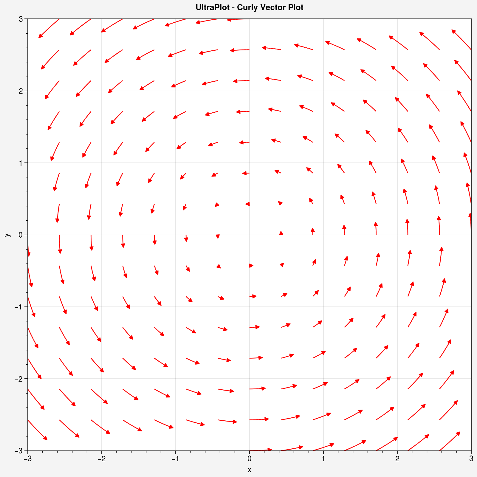
Ultraplot arguments:

• x, y = Grid coordinates

• u, v = Vector components

• color = color of the arrows

• density = controls how dense the arrows are displayed as

• grains = number of seed points in x and y

• linewidth = width of arrows

• cmap, norm = colormap and normalization for array colors

• colorbar = add colorbar

• arrowsize = arrow size

• arrowstyle = arrow style

• transform = Matplotlib transform

Working with Cartopy

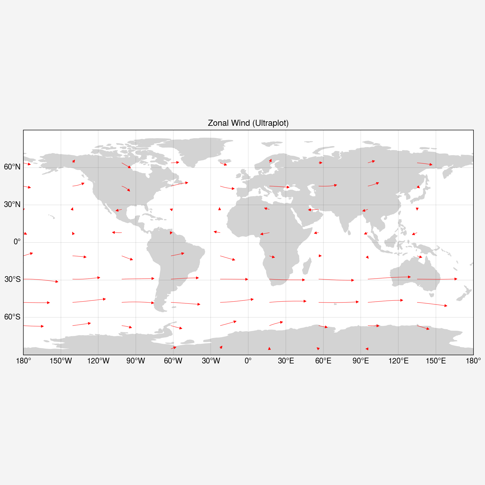
ultraplot can also overlay curly vector plots on top of world maps

Plot Vectors Globally

import geocat.datafiles as gdf  # NetCDF data files
import xarray as xr  # multi-dimensional arrays from data files

import matplotlib.pyplot as plt  # plotting
import cartopy  # plotting world maps
import ultraplot as uplot  # plotting curly vectors

# Open a netCDF data file using xarray default engine and load the data into xarrays
file_in = xr.open_dataset(gdf.get("netcdf_files/uv300.nc"))
ds = file_in.isel(time=1, lon=slice(0, -1, 3), lat=slice(1, -1, 3))

# plot
fig, ax = uplot.subplot(figsize=(8, 8), proj="cyl")

ax.add_feature(
    cartopy.feature.LAND, edgecolor='lightgray', facecolor='lightgray', zorder=0
)

ax.curved_quiver(
    ds['lon'].values,
    ds['lat'].values,
    ds['U'].values,
    ds['V'].values,
    color="red",
    arrow_at_end=True,
    arrowsize=0.7,
    linewidth=0.4,
    density=10,
    grains=10,
)

ax.format(
    land=False,
    lonlabels='bottom',  # place labels on the bottom (longitude)
    latlabels='left',  # place labels on the left (latitude)
    lonlocator=30,  # Labels every 30 degrees (longitude)
    latlocator=30,  # Labels every 30 degrees (latitude)
    lonformatter='deglon',  # Format to degrees East/West
    latformatter='deglat',  # Format to degrees North/South
)

plt.title("Zonal Wind (Ultraplot)")
plt.show()

Downloading file 'registry.txt' from 'https://github.com/NCAR/geocat-datafiles/raw/main/registry.txt' to '/home/runner/.cache/geocat'.

Downloading file 'netcdf_files/uv300.nc' from 'https://github.com/NCAR/geocat-datafiles/raw/main/netcdf_files/uv300.nc' to '/home/runner/.cache/geocat'.

/home/runner/micromamba/envs/geocat-applications/lib/python3.14/site-packages/cartopy/io/__init__.py:242: DownloadWarning: Downloading: https://naturalearth.s3.amazonaws.com/110m_physical/ne_110m_land.zip
  warnings.warn(f'Downloading: {url}', DownloadWarning)

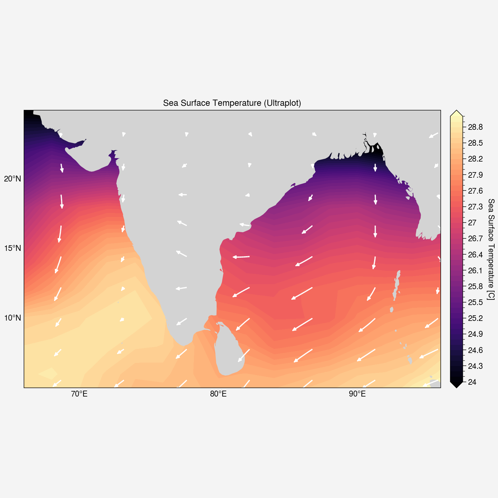
Plot Vectors on Sub-Set of Globe

import geocat.datafiles as gdf  # NetCDF data files
import xarray as xr  # multi-dimensional arrays from data files

import matplotlib.pyplot as plt  # plotting
import cartopy  # plotting world maps
import ultraplot as uplot  # plotting curly vectors

# Open a netCDF data file using xarray default engine and load the data into xarrays
sst_in = xr.open_dataset(gdf.get("netcdf_files/sst8292.nc"))
uv_in = xr.open_dataset(gdf.get("netcdf_files/uvt.nc"))

# Use date as the dimension rather than time
sst_in = sst_in.set_coords("date").swap_dims({"time": "date"}).drop_vars('time')
uv_in = uv_in.set_coords("date").swap_dims({"time": "date"}).drop_vars('time')

# Extract required variables
# Read SST and U, V for Jan 1988 (at 1000 mb for U, V)
# Note that we could use .isel() if we know the indices of date and lev
sst = sst_in['SST'].sel(date=198801)
u = uv_in['U'].sel(date=198801, lev=1000)
v = uv_in['V'].sel(date=198801, lev=1000)

# Read in grid information
lat_uv = u['lat']
lon_uv = u['lon']

# plot
fig, ax = uplot.subplot(figsize=(8, 8), proj="cyl")
ax.set_extent((66, 96, 5, 25))  # zoom on India

# Create the filled contour plot with "magma"
sst_plot = sst.plot.contourf(
    ax=ax,
    transform="cyl",
    levels=51,
    vmin=24,
    vmax=29,
    cmap="magma",
)

ax.add_feature(
    cartopy.feature.LAND, edgecolor='lightgray', facecolor='lightgray', zorder=1
)

ax.curved_quiver(
    lon_uv.values,
    lat_uv.values,
    u.values,
    v.values,
    color="white",
    arrow_at_end=True,
    arrowsize=0.7,
    linewidth=1.4,
    density=80,
    grains=80,
)

ax.format(
    title="Sea Surface Temperature (Ultraplot)",
    land=False,
    grid=False,
    lonlabels='bottom',  # place labels on the bottom (longitude)
    latlabels='left',  # place labels on the left (latitude)
    lonlocator=10,  # Labels every 10 degrees (longitude)
    latlocator=5,  # Labels every 5 degrees (latitude)
    lonformatter='deglon',  # Format to degrees East/West
    latformatter='deglat',  # Format to degrees North/South
)

plt.show()

Downloading file 'netcdf_files/sst8292.nc' from 'https://github.com/NCAR/geocat-datafiles/raw/main/netcdf_files/sst8292.nc' to '/home/runner/.cache/geocat'.

Downloading file 'netcdf_files/uvt.nc' from 'https://github.com/NCAR/geocat-datafiles/raw/main/netcdf_files/uvt.nc' to '/home/runner/.cache/geocat'.

/home/runner/micromamba/envs/geocat-applications/lib/python3.14/site-packages/cartopy/io/__init__.py:242: DownloadWarning: Downloading: https://naturalearth.s3.amazonaws.com/50m_physical/ne_50m_land.zip
  warnings.warn(f'Downloading: {url}', DownloadWarning)

Curated Resources

• NCL-inspired curly vectors: Skyborn

• GeoCAT-examples: Vector Plots