Getting Started#
Build and Test#
Configuring for different platforms and environments is shown here. There is an additional tutorial which covers some other specifics: Installation and usage.
CPU#
To build and install MICM locally, you must have the following libraries installed:
Then, it’s enough for you to configure and install micm on your computer. Because micm is header-only library, the install step will simply copy the header files into the normal location required by your system.
$ git clone https://github.com/NCAR/micm.git
$ cd micm
$ mkdir build
$ cd build
$ ccmake ..
$ make install -j 8
$ make test
CMake will allow for setting options such as the installation directory with CMAKE_INSTALL_PREFIX, or various build flags such as MICM_BUILD_DOCS, MICM_GPU_TYPE, etc.
Options#
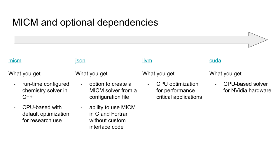
MICM can optionally include support for yaml configuration reading, OpenMP, and GPUs. Each of these requires an additional library. Some of these libraries can be included automatically with cmake build options, others require that you have libraries installed on your system.
GPU support - Coming soon
OpenMP - On macOS, you either need to configure cmake to use gcc which ships with OpenMP (either
CXX=g++ cmake -DMICM_ENABLE_OPENMP=ON ..orcmake -DCMAKE_CXX_COMPILER=g++ -DMICM_ENABLE_OPENMP=ON ..)
For more ways to build and install micm, see Installation and usage. If you would like instructions for building the docs, see Contributing.
Docker Container#
Build and run the image:
$ docker build -t micm -f docker/Dockerfile.nvhpc .
$ docker run --rm -it micm
If you would like, you can ssh into a running docker container and edit the files there.
Run an Example#
MICM API Example#
The following example solves the fictitious chemical system:
foo       --k1--> 0.8 bar + 0.2 baz
foo + bar --k2--> baz
The k1 and k2 rate constants are for Arrhenius reactions. See the MICM documentation <https://ncar.github.io/micm/> for details on the types of reactions available in MICM and how to configure them. To solve this system save the following code in a file named foo_chem.cpp
#include <micm/CPU.hpp>

#include <iomanip>
#include <iostream>

using namespace micm;

int main(const int argc, const char *argv[])
{
  auto foo = Species{ "Foo" };
  auto bar = Species{ "Bar" };
  auto baz = Species{ "Baz" };

  Phase gas_phase{ "gas", std::vector<PhaseSpecies>{ foo, bar, baz } };

  System chemical_system{ SystemParameters{ .gas_phase_ = gas_phase } };

  Process r1 = ChemicalReactionBuilder()
                   .SetReactants({ foo })
                   .SetProducts({ StoichSpecies(bar, 0.8), StoichSpecies(baz, 0.2) })
                   .SetRateConstant(ArrheniusRateConstant({ .A_ = 1.0e-3 }))
                   .SetPhase(gas_phase)
                   .Build();

  Process r2 = ChemicalReactionBuilder()
                   .SetReactants({ foo, bar })
                   .SetProducts({ StoichSpecies(baz, 1) })
                   .SetRateConstant(ArrheniusRateConstant({ .A_ = 1.0e-5, .C_ = 110.0 }))
                   .SetPhase(gas_phase)
                   .Build();

  std::vector<Process> reactions{ r1, r2 };

  auto solver = micm::CpuSolverBuilder<micm::RosenbrockSolverParameters>(
                    micm::RosenbrockSolverParameters::ThreeStageRosenbrockParameters())
                    .SetSystem(chemical_system)
                    .SetReactions(reactions)
                    .Build();

  State state = solver.GetState();

  state.conditions_[0].temperature_ = 287.45;  // K
  state.conditions_[0].pressure_ = 101319.9;   // Pa
  state.conditions_[0].CalculateIdealAirDensity();
  state.SetConcentration(foo, 20.0);  // mol m-3

  state.PrintHeader();
  for (int i = 0; i < 10; ++i)
  {
    solver.CalculateRateConstants(state);
    auto result = solver.Solve(500.0, state);
    state.PrintState(i * 500);
  }

  return 0;
}
To build and run the example using GNU:
$ g++ -o foo_chem foo_chem.cpp -I<CMAKE_INSTALL_PREFIX>/include -std=c++20
$ ./foo_chem
You should see an output including this
time [s] |
foo |
bar |
baz |
|---|---|---|---|
0.000000 |
11.843503 |
5.904845 |
1.907012 |
500.000000 |
6.792023 |
9.045965 |
3.317336 |
1000.000000 |
3.828700 |
10.740589 |
4.210461 |
1500.000000 |
2.138145 |
11.663685 |
4.739393 |
2000.000000 |
1.187934 |
12.169452 |
5.042503 |
2500.000000 |
0.658129 |
12.447502 |
5.213261 |
3000.000000 |
0.363985 |
12.600676 |
5.308597 |
3500.000000 |
0.201076 |
12.685147 |
5.361559 |
4000.000000 |
0.111028 |
12.731727 |
5.390884 |
4500.000000 |
0.061290 |
12.757422 |
5.407096 |