Python#

1. Installing MUSICA#

To install MUSICA onto your device, run

$ pip install musica

2. Importing MUSICA#

To import your newly-downloaded MUSICA, as well as some other libraries for this demo, into a Python file,

import musica
import musica.mechanism_configuration as mc
import matplotlib.pyplot as plt
import pandas as pd

3. Define the chemical system of interest#

In MUSICA, a system is defined by a mechanism that includes:

a set of species and their respective phases, and
a set of reactions that the species participate in.

The system is the fundamental building block of MUSICA. The following steps will walk you through:

creating your own system,
solving your system, and
viewing and visualizing your results.

3a. Defining species#

A species is a reactant or product in a chemical reaction. You have the freedom to name a species anything in MusicBox, just make sure that it is logical to you. For extended documentation about the Species class, go here.

Here is a snippet that defines three chemical species:

A = mc.Species(name="A")
B = mc.Species(name="B")
C = mc.Species(name="C")
species = [A, B, C]
gas = mc.Phase(name="gas", species=species)

3b. Define a mechanism of interest#

Through MUSICA, several different mechanisms can be explored to define reaction rates. Here, we use the Arrhenius equation as a simple example:

r1 = mc.Arrhenius(name="A->B", A=4.0e-3, C=50, reactants=[A], products=[B], gas_phase=gas)
r2 = mc.Arrhenius(name="B->C", A=1.2e-4, B=2.5, C=75, D=50, E=0.5, reactants=[B], products=[C], gas_phase=gas)

mechanism = mc.Mechanism(name="musica_example", species=species, phases=[gas], reactions=[r1, r2])

This code block uses the gas and species variables from the previous section. Using the species and gas variables, it creates two reactions: r1 and r2. The r1 variable represents the conversion of A (reactant) into B (product) and defines Arrhenius rate constant parameters A and C. The r2 variable is just like arr1, but instead it represents the conversion of B (reactant) into C (product). More information on the Arrhenius reaction can be found here. Go here to view a list of supported reactions and their parameters.

4. Create MICM solver#

A solver must be initialized with either a configuration file or a mechanism, and it integrates the chemical reactions that determine how atmospheric chemistry proceeds over time. There are a handful of solvers available, but Rosenbrock Standard Order is used here:

solver = musica.MICM(mechanism=mechanism, solver_type=musica.SolverType.rosenbrock_standard_order)

For more information on the types of solvers available, see the MICM User Guide.

5. Define environmental conditions#

MUSICA supports the definition of initial conditions that define the environment that the mechanism takes place in at the start of the simulation:

temperature=300.0 # Kelvin
pressure=101000.0 #Pascals

6. Create and initialize State#

In the model, conditions are assigned by modifying the state:

state = solver.create_state()
state.set_concentrations({"A": 1.0, "B": 3.0, "C": 5.0})
state.set_conditions(temperature, pressure)

Note that concentrations are in mol/m<sup>3</sup>

7. Time parameters#

Below, we define both the total time span of the simulation and the size of each timestep used to iterate through it:

time_step = 4  # stepping
sim_length = 20  # total simulation time

8. (Optional) Save initial state (t=0) for output visualization#

For later visualization, it is helpful to store the conditions with which your model began:

initial_row = {"time.s": 0.0, "ENV.temperature.K": temperature, "ENV.pressure.Pa": pressure, "ENV.air number density.mol m-3": state.get_conditions()['air_density'][0]}
initial_row.update({f"CONC.{k}.mol m-3": v[0] for k, v in state.get_concentrations().items()})

9. Solve through time loop only#

This code solves the system at every specified time step:

curr_time = time_step
while curr_time <= sim_length:
    solver.solve(state, time_step)
    concentrations = state.get_concentrations()
    curr_time += time_step

10. Solve and create DataFrame#

It is likely more useful to solve at each time step and store the associated data:

output_data = [] # prepare to store output per time step
output_data.append(initial_row) # save t=0 data

curr_time = time_step
while curr_time <= sim_length:
    solver.solve(state, time_step)
    row = {
        "time.s": curr_time,
        "ENV.temperature.K": state.get_conditions()['temperature'][0],
        "ENV.pressure.Pa": state.get_conditions()['pressure'][0],
        "ENV.air number density.mol m-3": state.get_conditions()['air_density'][0]
    }
    row.update({f"CONC.{k}.mol m-3": v[0] for k, v in state.get_concentrations().items()})
    output_data.append(row)
    curr_time += time_step

df = pd.DataFrame(output_data)
print(df)

11. Visualize specific results#

With a DataFrame now prepared and filled with the simulation results, it can be displayed and plotted to show the evolution of one of the systems over time:

df.plot(x='time.s', y=['CONC.A.mol m-3', 'CONC.B.mol m-3', 'CONC.C.mol m-3'], title='Concentration over time', ylabel='Concentration (mol m-3)', xlabel='Time (s)')
plt.show()

	time.s	ENV.temperature.K	ENV.pressure.Pa	ENV.air number density.mol m-3	CONC.A.mol m-3	CONC.B.mol m-3	CONC.C.mol m-3
0	0	300	101000	40.4917	1	3	5
1	4	300	101000	40.4917	0.892784	6.14835e-06	8.10721
2	8	300	101000	40.4917	0.876067	6.03323e-06	8.12393
3	12	300	101000	40.4917	0.859664	5.92026e-06	8.14033
4	16	300	101000	40.4917	0.843567	5.80941e-06	8.15643
5	20	300	101000	40.4917	0.827772	5.70063e-06	8.17222

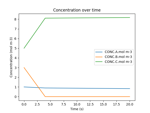
This code block prints out the output of the simulation that was just ran as well as utilizing Python’s matplotlib library to visualize it. To do so, the plot() function is called, with the desired independent variable (time) and dependent variables (concentration of each species) being passed in. The plot is also given a title as well as a label for both the x-axis and the y-axis. Lastly, the show() function is called so that you can see the plot directly above this text.