Output and visualization

MUSICA simulation results can be stored and visualized with the use of Pandas and Matplotlib. However, these packages are not direct dependencies of MUSICA and must be installed for users wishing to visualize their MUSICA results in this manner.

Installing pandas and matplotlib

Both pandas and matplotlib are pip installable and can be installed in your conda environment created for MUSICA with:

pip install pandas
pip install matplotlib

They can then be used in any Python script with the following import statement:

import pandas as pd
import matplotlib.pyplot as plt

Note that ‘pd’ and ‘plt’ are used to shorten the name of pandas and matplotlib.pyplot, but the user can specify any nickname.

Storing MUSICA results

After a state is created in MUSICA, the initial conditions should be saved in order to record the time = 0 environment of your simulation:

initial_row = {"time.s": 0.0, "ENV.temperature.K": temperature, "ENV.pressure.Pa": pressure, "ENV.air number density.mol m-3": state.get_conditions()['air_density'][0]}
initial_row.update({f"CONC.{k}.mol m-3": v[0] for k, v in state.get_concentrations().items()})

With the intention of storing the resulting data at each time step, the model solving loop can be modified to append the results to lists to later be turned into a pandas DataFrame:

output_data = [] # prepare to store output per time step
output_data.append(initial_row) # save t=0 data

curr_time = time_step
while curr_time <= sim_length:
    solver.solve(state, time_step)
    row = {
        "time.s": curr_time,
        "ENV.temperature.K": state.get_conditions()['temperature'][0],
        "ENV.pressure.Pa": state.get_conditions()['pressure'][0],
        "ENV.air number density.mol m-3": state.get_conditions()['air_density'][0]
    }
    row.update({f"CONC.{k}.mol m-3": v[0] for k, v in state.get_concentrations().items()})
    output_data.append(row)
    curr_time += time_step

df = pd.DataFrame(output_data)

Visualizing MUSICA results

This dataframe can be visualized as-is with:

print(df)

	time.s	ENV.temperature.K	ENV.pressure.Pa	ENV.air number density.mol m-3	CONC.X.mol m-3	CONC.Y.mol m-3	CONC.Z.mol m-3
0	0	300	101000	40.4917	1	3	5
1	4	300	101000	40.4917	0.892784	6.14835e-06	8.10721
2	8	300	101000	40.4917	0.876067	6.03323e-06	8.12393
3	12	300	101000	40.4917	0.859664	5.92026e-06	8.14033
4	16	300	101000	40.4917	0.843567	5.80941e-06	8.15643
5	20	300	101000	40.4917	0.827772	5.70063e-06	8.17222

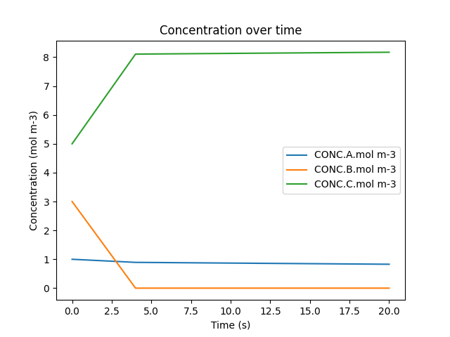
Or specific concentrations can be visualized in a plot as follows:

df.plot(x='time.s', y=['CONC.X.mol m-3', 'CONC.Y.mol m-3', 'CONC.Z.mol m-3'], title='Concentration over time', ylabel='Concentration (mol m-3)', xlabel='Time (s)')
plt.show()