Bias-correct CESM2 LENS temperature data using ERA5 reanalysis

Input Data Access¶

This notebook illustrates how to bias-correct daily temperature data from CESM2 Large Ensemble Dataset (https://www.cesm.ucar.edu/community-projects/lens2) hosted on AWS.
This data is open access (https://aws.amazon.com/marketplace/pp/prodview-xilranwbl2ep2#resources)
We will access the data using OSDF’s AWS open data origin.
The OSDF zarr paths are obtained from an intake catalog which lives on NCAR’s Geoscience Data Exchange (GDEX) and is publicly accessible via https.
We will use NCAR’s origin to access the publicly available ERA5 reanalysis.
In summary, this notebook illustrates how we can access data from two different OSDF origins using PelicanFS and perform an interesting computation.

Computational resources and Output data¶

If you don’t have access to NCAR’s HPC system, please select the appropriate cluster
All the intermediate results and the final result will be written to NCAR’s GLADE storage system, which doesn’t have public write access.
You are welcome to modify this to suit your needs.

Import package, define parameters and functions¶

# Imports
import intake
import numpy as np
import pandas as pd
import xarray as xr
# import s3fs
import seaborn as sns
import re
# import xesmf as xe   # Note: Avoiding the use of xesmf as it depends on ESMPy which isn't available via PyPI (pip)
import xarray_regrid   # Instead, use xarray_regrid 
import matplotlib.pyplot as plt
# import cartopy as cart

import fsspec.implementations.http as fshttp
from pelicanfs.core import PelicanFileSystem, PelicanMap, OSDFFileSystem

import dask 
from dask_jobqueue import PBSCluster
from dask.distributed import Client
from dask.distributed import performance_report

init_year0  = '1991'
init_year1  = '2020'
final_year0 = '2071'
final_year1 = '2100'

def to_daily(ds):
    year = ds.time.dt.year
    day = ds.time.dt.dayofyear

    # assign new coords
    ds = ds.assign_coords(year=("time", year.data), day=("time", day.data))

    # reshape the array to (..., "day", "year")
    return ds.set_index(time=("year", "day")).unstack("time")

lustre_scratch   = "/lustre/desc1/scratch/harshah"
zarr_path   = "/gdex/scratch/harshah/tas_zarr/"
mean_path   = zarr_path + "/means/"
stdev_path  = zarr_path + "/stdevs/"
#
catalog_url = 'https://data-osdf.gdex.ucar.edu/ncar-gdex/d010092/catalogs/d010092-osdf-zarr.json' 
# catalog_url = 'https://stratus.gdex.ucar.edu/d010092/catalogs/d010092-https-zarr.json'

Create a Dask cluster¶

Dask Introduction¶

Dask is a solution that enables the scaling of Python libraries. It mimics popular scientific libraries such as numpy, pandas, and xarray that enables an easier path to parallel processing without having to refactor code.

There are 3 components to parallel processing with Dask: the client, the scheduler, and the workers.

The Client is best envisioned as the application that sends information to the Dask cluster. In Python applications this is handled when the client is defined with client = Client(CLUSTER_TYPE). A Dask cluster comprises of a single scheduler that manages the execution of tasks on workers. The CLUSTER_TYPE can be defined in a number of different ways.

There is LocalCluster, a cluster running on the same hardware as the application and sharing the available resources, directly in Python with dask.distributed.
In certain JupyterHubs Dask Gateway may be available and a dedicated dask cluster with its own resources can be created dynamically with dask.gateway.
On HPC systems dask_jobqueue is used to connect to the HPC Slurm, PBS or HTCondor job schedulers to provision resources.

The dask.distributed client python module can also be used to connect to existing clusters. A Dask Scheduler and Workers can be deployed in containers, or on Kubernetes, without using a Python function to create a dask cluster. The dask.distributed Client is configured to connect to the scheduler either by container name, or by the Kubernetes service name.

Select the Dask cluster type¶

The default will be LocalCluster as that can run on any system.

If running on a HPC computer with a PBS Scheduler, set to True. Otherwise, set to False.

USE_PBS_SCHEDULER = True

If running on Jupyter server with Dask Gateway configured, set to True. Otherwise, set to False.

USE_DASK_GATEWAY = False

Python function for a PBS cluster¶

# Create a PBS cluster object
def get_pbs_cluster():
    """ Create cluster through dask_jobqueue.   
    """
    from dask_jobqueue import PBSCluster
    cluster = PBSCluster(
        job_name = 'dask-osdf-24',
        cores = 1,
        memory = '4GiB',
        processes = 1,
        local_directory = lustre_scratch + '/dask/spill',
        log_directory = lustre_scratch + '/dask/logs/',
        resource_spec = 'select=1:ncpus=1:mem=4GB',
        queue = 'casper',
        walltime = '3:00:00',
        #interface = 'ib0'
        interface = 'ext'
    )
    return cluster

Python function for a Gateway Cluster¶

def get_gateway_cluster():
    """ Create cluster through dask_gateway
    """
    from dask_gateway import Gateway

    gateway = Gateway()
    cluster = gateway.new_cluster()
    cluster.adapt(minimum=2, maximum=4)
    return cluster

Python function for a Local Cluster¶

def get_local_cluster():
    """ Create cluster using the Jupyter server's resources
    """
    from distributed import LocalCluster, performance_report
    cluster = LocalCluster()    

    cluster.scale(4)
    return cluster

Python logic to select the Dask Cluster type¶

This uses True/False boolean logic based on the variables set in the previous cells

# Obtain dask cluster in one of three ways

if USE_PBS_SCHEDULER:
    cluster = get_pbs_cluster()
elif USE_DASK_GATEWAY:
    cluster = get_gateway_cluster()
else:
    cluster = get_local_cluster()

# Connect to cluster
from distributed import Client
client = Client(cluster)

/glade/u/home/harshah/venvs/osdf/lib/python3.10/site-packages/distributed/node.py:187: UserWarning: Port 8787 is already in use.
Perhaps you already have a cluster running?
Hosting the HTTP server on port 42145 instead
  warnings.warn(

# Scale the cluster and display cluster dashboard URL
cluster.scale(4)

cluster

Load CESM LENS2 temperature data from AWS using an intake catalog¶

cesm_cat = intake.open_esm_datastore(catalog_url)
cesm_cat

cesm_temp = cesm_cat.search(variable ='TREFHTMX', frequency ='daily')
cesm_temp

cesm_temp.df['path'].values

array(['https://stratus.gdex.ucar.edu/d010092/atm/daily/cesm2LE-historical-cmip6-TREFHTMX.zarr',
       'https://stratus.gdex.ucar.edu/d010092/atm/daily/cesm2LE-historical-smbb-TREFHTMX.zarr',
       'https://stratus.gdex.ucar.edu/d010092/atm/daily/cesm2LE-ssp370-cmip6-TREFHTMX.zarr',
       'https://stratus.gdex.ucar.edu/d010092/atm/daily/cesm2LE-ssp370-smbb-TREFHTMX.zarr'],
      dtype=object)

%%time
dsets_cesm = cesm_temp.to_dataset_dict()

historical_smbb  = dsets_cesm['atm.historical.daily.smbb']
future_smbb      = dsets_cesm['atm.ssp370.daily.smbb']

historical_cmip6 = dsets_cesm['atm.historical.daily.cmip6']
future_cmip6     = dsets_cesm['atm.ssp370.daily.cmip6']

historical_smbb_init = historical_smbb.TREFHTMX.sel(time=slice(init_year0, init_year1))
historical_smbb_init

%%time
# Plot sample data
historical_smbb.TREFHTMX.isel(member_id=0,time=0).plot()

CPU times: user 141 ms, sys: 15.4 ms, total: 156 ms
Wall time: 1.01 s

# %%time
# merge_ds_smbb = xr.concat([historical_smbb, future_smbb], dim='time')
# merge_ds_smbb = merge_ds_smbb.dropna(dim='member_id')

# merge_ds_cmip6= xr.concat([historical_cmip6, future_cmip6], dim='time')
# merge_ds_cmip6 = merge_ds_cmip6.dropna(dim='member_id')

# t_smbb      = merge_ds_smbb.TREFHTMX
# t_cmip6     = merge_ds_cmip6.TREFHTMX
# t_init_cmip6 = t_cmip6.sel(time=slice(init_year0, init_year1))
# t_init_smbb  = t_smbb.sel(time=slice(init_year0, init_year1))
# t_init       = xr.concat([t_init_cmip6,t_init_smbb],dim='member_id')
# t_init

# t_init_day = to_daily(t_init)
# #t_init_day

# t_fut_cmip6 = t_cmip6.sel(time=slice(final_year0, final_year1))
# t_fut_smbb  = t_smbb.sel(time=slice(final_year0, final_year1))
# t_fut       = xr.concat([t_fut_cmip6,t_fut_smbb],dim='member_id')
# t_fut_day   = to_daily(t_fut)
# t_fut_day

Save means and standard deviations¶

# init_means   = t_init_day.mean({'year','member_id'})
# init_stdevs  = t_init_day.std({'year','member_id'})
# final_means  = t_fut_day.mean({'year','member_id'})
# final_stdevs = t_fut_day.std({'year','member_id'})
#
# init_ensemble_means  = t_init_day.mean({'member_id'})
# final_ensemble_means = t_fut_day.mean({'member_id'})
# init_ensemble_means  = init_ensemble_means.chunk({'lat':192,'lon':288,'year':2,'day':365})
# final_ensemble_means = final_ensemble_means.chunk({'lat':192,'lon':288,'year':2,'day':365})

Save the overall means, standard devaitions and the ensemble means
We will regrid the ‘final/EOC’ ensemble means onto the ERA5 grid.
We will then compare it with the bias-corrected future predictions obtained from ERA5

# %%time
# init_means.to_dataset().to_zarr(mean_path + 'cesm2_'+ init_year0 + '_' + init_year1+ '_means.zarr',mode='w')
# init_stdevs.to_dataset().to_zarr(stdev_path + 'cesm2_'+ init_year0 + '_' + init_year1+ '_stdevs.zarr',mode='w') 
# final_means.to_dataset().to_zarr(mean_path + 'cesm2_'+ final_year0 + '_' + final_year1+ '_means.zarr',mode='w')
# final_stdevs.to_dataset().to_zarr(stdev_path + 'cesm2_'+ final_year0 + '_' + final_year1+ '_stdevs.zarr',mode='w') 
# init_ensemble_means.to_dataset().to_zarr(mean_path + 'cesm2_'+ init_year0 + '_' + init_year1 \
#                                          + '_ensemble_means.zarr',mode='w')
# final_ensemble_means.to_dataset().to_zarr(mean_path + 'cesm2_'+ final_year0 + '_' + final_year1 \
#                                           + '_ensemble_means.zarr',mode='w')

Access ERA5 data and regrid CESM2 LENS data on the finer, ERA5 grid¶

In this section, we will load pre-processed ERA5 data from the NCAR origin
We will not use an intake catalog

# Create OSDF file path for the ERA5 zarr store
namespace        = 'ncar/'   #NCAR's GDEX
# osdf_director    = 'https://osdf-director.osg-htc.org/'
osdf_director    = 'osdf:///'
era5_zarr_path   = namespace + 'gdex/special_projects/harshah/era5_tas/zarr/e5_tas2m_daily_1940_2023.zarr'
#
# osdf_fs = OSDFFileSystem()
print(era5_zarr_path)
osdf_protocol_era5path = osdf_director + era5_zarr_path
print(osdf_protocol_era5path)

ncar/gdex/special_projects/harshah/era5_tas/zarr/e5_tas2m_daily_1940_2023.zarr
osdf:///ncar/gdex/special_projects/harshah/era5_tas/zarr/e5_tas2m_daily_1940_2023.zarr

%%time
tas_obs_daily = xr.open_zarr(osdf_protocol_era5path).VAR_2T
tas_obs_init = tas_obs_daily.sel(time=slice(init_year0, init_year1))
tas_obs_init

Perform Bias Correction¶

init_means_ds = xr.open_zarr(mean_path + 'cesm2_'+ init_year0 + '_' + init_year1+ '_means.zarr')
init_means    = init_means_ds.TREFHTMX
init_means

final_means  = xr.open_zarr(mean_path  + 'cesm2_'+ final_year0 + '_' + final_year1+ '_means.zarr').TREFHTMX
init_stdevs  = xr.open_zarr(stdev_path + 'cesm2_'+ init_year0 + '_' + init_year1+ '_stdevs.zarr').TREFHTMX
final_stdevs = xr.open_zarr(stdev_path + 'cesm2_'+ final_year0 + '_' + final_year1+ '_stdevs.zarr').TREFHTMX

tas_obs_initial    = to_daily(tas_obs_init)
tas_obs_initial    = tas_obs_initial.rename({'latitude':'lat','longitude':'lon'})
tas_obs_initial    = tas_obs_initial.chunk({'lat':139,'lon':544,'year':3,'day':90})
tas_obs_initial

# %%time
# tas_obs_initial.to_dataset().to_zarr(zarr_path + "e5_tas2m_initial_1991_2020.zarr",mode='w')

tas_obs_initial = xr.open_zarr(zarr_path + "e5_tas2m_initial_1991_2020.zarr").VAR_2T

Re-grid the model data onto the ERA5 grid¶

Using xesmf¶

# #Create output grid
# ds_out = xr.Dataset(
#     coords={
#         'latitude': tas_obs_init.coords['latitude'],
#         'longitude': tas_obs_init.coords['longitude']
#     }
# )
# ds_out = ds_out.rename({'latitude':'lat','longitude':'lon'})
# ds_out

# %%time 
# regridder = xe.Regridder(init_means_ds, ds_out, "bilinear")
# regridder

# init_means_regrid = regridder(init_means, keep_attrs=True)
# init_means_regrid

# %%time
# # Regrid other variables
# init_stdevs_regrid  = regridder(init_stdevs, keep_attrs=True)
# final_means_regrid  = regridder(final_means, keep_attrs=True)
# final_stdevs_regrid = regridder(final_stdevs, keep_attrs=True)

Using xarray-regridder¶

#Create output grid
ds_target = xr.Dataset(
    coords={
        'latitude': tas_obs_init.coords['latitude'],
        'longitude': tas_obs_init.coords['longitude']
    }
)
ds_target = ds_target.rename({'latitude':'lat','longitude':'lon'})
ds_target

%%time
# Regrid variables
init_means_regrid   = init_means.regrid.nearest(ds_target)
init_stdevs_regrid  = init_stdevs.regrid.nearest(ds_target)
final_means_regrid  = final_means.regrid.nearest(ds_target)
final_stdevs_regrid = final_stdevs.regrid.nearest(ds_target)

CPU times: user 863 ms, sys: 37 ms, total: 900 ms
Wall time: 986 ms

# %%time
# #Save regridded data
# init_means_regrid.to_dataset().to_zarr(mean_path + 'cesm2_'+ init_year0 + '_' + init_year1+ '_means_regridded.zarr',mode='w')
# init_stdevs_regrid.to_dataset().to_zarr(stdev_path + 'cesm2_'+ init_year0 + '_' + init_year1+ '_stdevs_regridded.zarr',mode='w') 
# final_means_regrid.to_dataset().to_zarr(mean_path + 'cesm2_'+ final_year0 + '_' + final_year1+ '_means_regridded.zarr',mode='w')
# final_stdevs_regrid.to_dataset().to_zarr(stdev_path + 'cesm2_'+ final_year0 + '_' + final_year1+ '_stdevs_regridded.zarr',mode='w')

%%time
# Open regridded data
init_means_regrid  = xr.open_zarr(mean_path + 'cesm2_'+ init_year0 + '_' + init_year1+ '_means_regridded.zarr').TREFHTMX
init_stdevs_regrid = xr.open_zarr(stdev_path + 'cesm2_'+ init_year0 + '_' + init_year1+ '_stdevs_regridded.zarr').TREFHTMX
final_means_regrid  = xr.open_zarr(mean_path + 'cesm2_'+ final_year0 + '_' + final_year1+ '_means_regridded.zarr').TREFHTMX
final_stdevs_regrid = xr.open_zarr(stdev_path + 'cesm2_'+ final_year0 + '_' + final_year1+ '_stdevs_regridded.zarr').TREFHTMX

CPU times: user 12.3 ms, sys: 109 μs, total: 12.4 ms
Wall time: 12.6 ms

Now, perform bias correction by only adjusting the first moment, i.e, mean and plot¶

tas_bc = tas_obs_initial  + (final_means_regrid - init_means_regrid)
tas_bc = tas_bc.chunk({'lat':139,'lon':544,'year':3,'day':90})
tas_bc

Plot bias corrected temperature and CESM model’s predictions for the End of the 21st century (2100)¶

Since tas_bc are predictions for the years 2070-2100, we need to change the year coordinated
We will then save the bias-corrected surface air temperatures (tas) to a zarr store.
Finally, we will read from this zarr store and plot

# Change the year coordinate
tas_bc['year'] = tas_bc['year'] + 80
tas_bc         = tas_bc.rename('bias_corrected_tas')
tas_bc

# %%time
# tas_bc.to_dataset().to_zarr(zarr_path + 'bias_corrected_tas_1991_2020.zarr',mode='w')

tas_bc = xr.open_zarr(zarr_path + 'bias_corrected_tas_1991_2020.zarr').bias_corrected_tas
tas_bc = tas_bc.sortby('lat',ascending=True)
tas_bc

final_ensemble_means = xr.open_zarr(mean_path + 'cesm2_'+ final_year0 + '_' + final_year1 + '_ensemble_means.zarr').TREFHTMX
final_ensemble_means = final_ensemble_means.sortby('lat',ascending=True)
final_ensemble_means

%%time
tas_bc.sel(year = 2100, day = 211).plot()

CPU times: user 226 ms, sys: 24 ms, total: 249 ms
Wall time: 880 ms

final_ensemble_means.sel(year = 2100, day = 211).plot()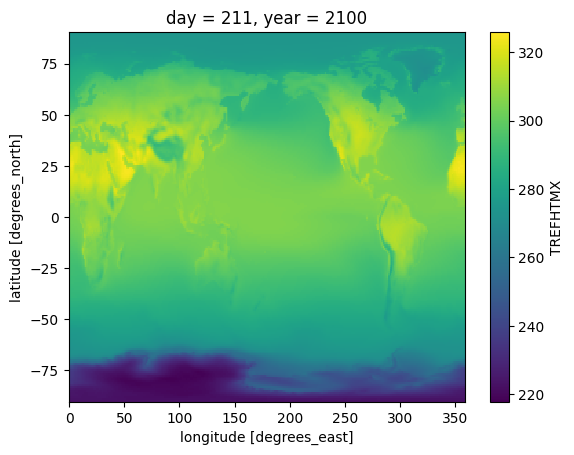

%%time
fig, axs = plt.subplots(1, 2, figsize=(10, 5))

# Plot the first array
tas_bc.sel(year = 2100, day = 211).plot(ax = axs[0],cmap='RdBu_r',add_colorbar=False)
axs[0].set_title('Bias-corrected projections')
#axs[0].coastlines(color="black")

# Plot the second array
final_ensemble_means.sel(year = 2100, day = 211).plot(ax = axs[1],cmap='RdBu_r')
axs[1].set_title('EOC model ensemble means')

# Display the plots
plt.show()

CPU times: user 1.01 s, sys: 68.6 ms, total: 1.08 s
Wall time: 1.5 s

cluster.close()

OSDF usage examples

Notebooks

Access CESM2 LENS data from NCAR’s Geoscience Data Exchange (GDEX) and compute GMST