Allison Baker (Jun 12 2020 at 17:46): Allison Baker (Jun 12 2020 at 17:46):
Hi all,
Plotting CAM-FV data seems pretty straightforward. I do something like this:
tsdata = ds.TS.isel(time=0)
latdata = ds.lat
londata = ds.lon
cy_tsdata, cy_londata = add_cyclic_point(tsdata, coord=ds['lon'])
fig = plt.figure(dpi=300)
mymap = cmocean.cm.thermal
ax = plt.axes(projection=ccrs.PlateCarree(central_longitude = 0.0, globe=None))
ctrf = ax.contourf(cy_londata, latdata, cy_tsdata, transform=ccrs.PlateCarree(), cmap=mymap, levels = 25)
But, I am having trouble with the SE data. I am doing this:
se_tsdata = se_ds.TS.isel(time=0)
se_latdata = se_ds.lat
se_londata = se_ds.lon
new_se_londata = np.where(se_londata > 180.0, se_londata - 360.0, se_londata)
se_fig = plt.figure(dpi=300)
se_mymap = cmocean.cm.thermal
se_ax = plt.axes(projection=ccrs.PlateCarree(central_longitude = 0.0, globe=None))
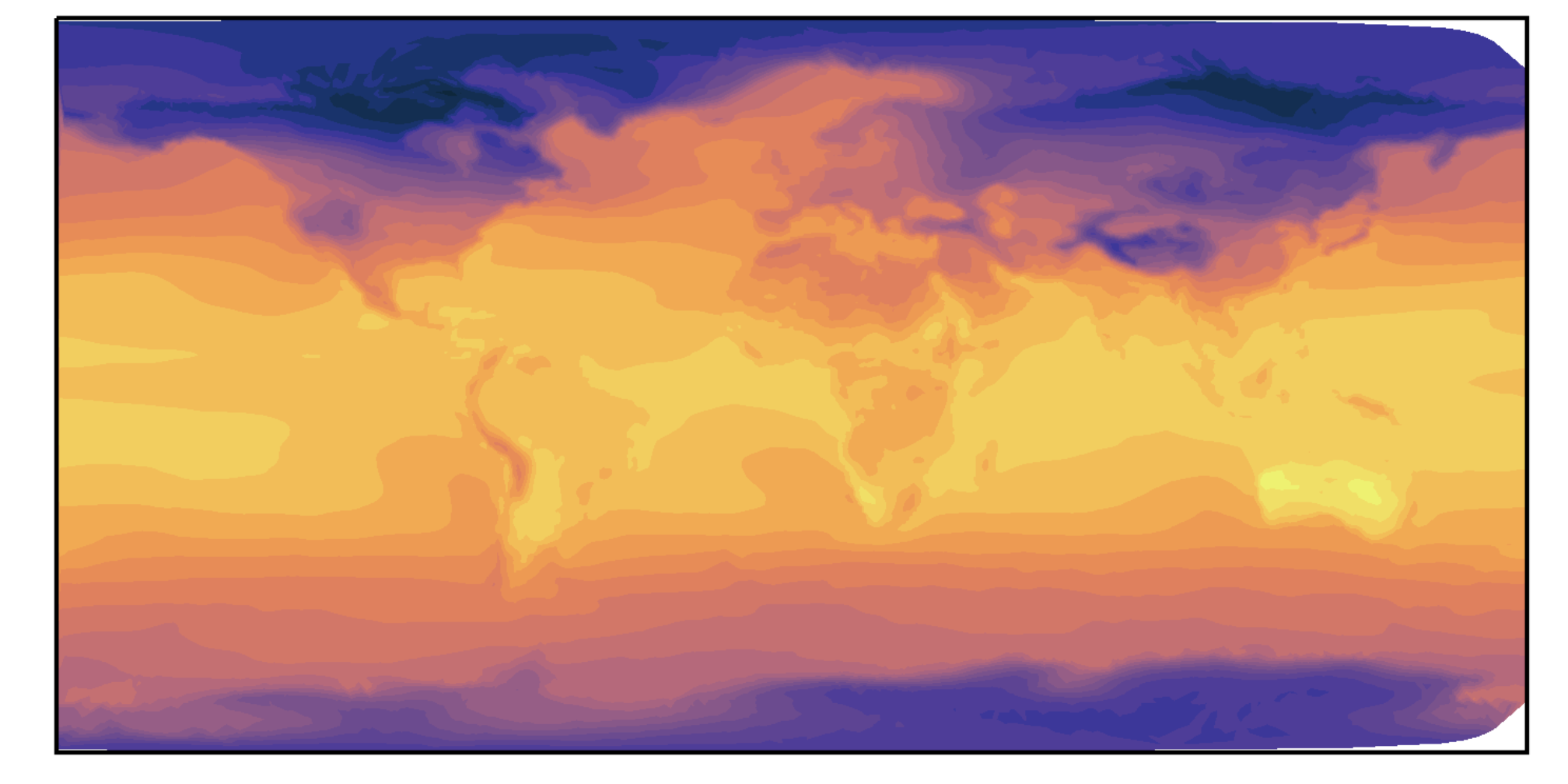
tcf = se_ax.tricontourf(new_se_londata, se_latdata, se_tsdata, cmap=se_mymap)
But now my plot has funny artifacts:
camse.png
Do I need to regrid first so that I can use contourf (instead of tricontourf). If anyone has advice or example code, I'd appreciate it!
Thanks! Allison
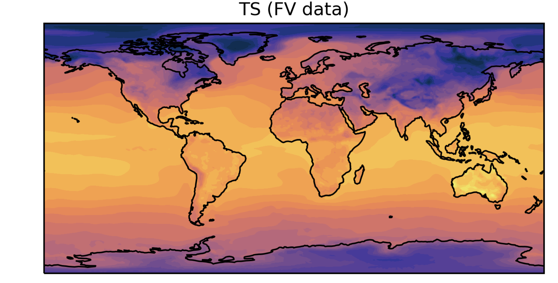
Michael Levy (Jun 12 2020 at 17:50):@Allison Baker can you attach the FV plot as well for comparison?
Allison Baker (Jun 12 2020 at 17:51):Here's the FV plot: fv-data.png
Allison Baker (Jun 12 2020 at 17:52):It's the white stuff in the upper and lower right corners that I don't know how to fix...
Michael Levy (Jun 12 2020 at 17:55):It's the white stuff in the upper and lower right corners that I don't know how to fix...
oh, gotcha -- I was expecting the issue to be cubed-sphere imprinting but didn't see it on the SE plot.
Kevin Paul (Jun 12 2020 at 17:58):Is this an artifact of tricontourf not knowing anything about cyclic coordinates?
Allison Baker (Jun 12 2020 at 19:22):hmmm..that is probably right. But I'm not sure how to do that without first regriding to a structured grid - which is probably what ncl does... I'm hoping there is an existing python option for this
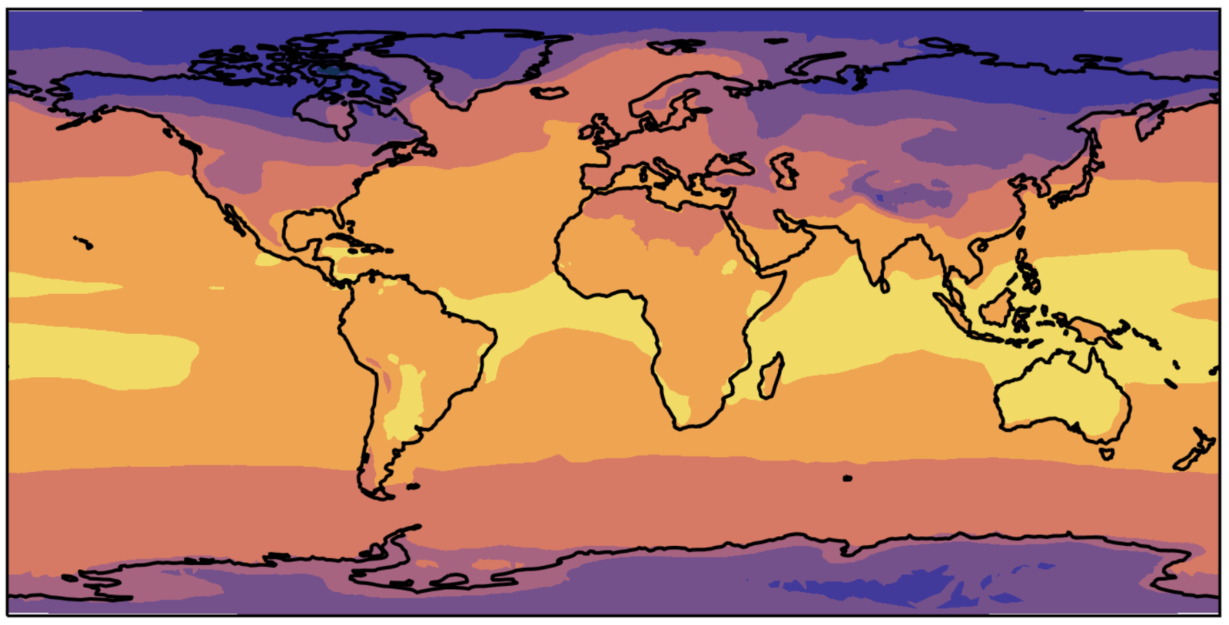
Kevin Paul (Jun 16 2020 at 22:00):@Allison Baker: I think I have a solution to your problem. I created a function to manually "fix" the cyclic coordinate. It is, at the moment, pretty specific to your problem (CESM-SE data with -180 < lon < 180), but it should work:
ds = xr.open_dataset('ihesp14.TS.12mon.nc')
ds.lon.data = np.where(ds.lon > 180.0, ds.lon - 360.0, ds.lon)    # fix data: -180 < lon < 180

# Retrieve reduced datasets corresponding to points on the lon==-180.0 and lon==+180.0 lines
ds_1 = ds.where(ds.lon < -179.9999).dropna(dim='ncol')
ds_2 = ds.where(ds.lon > 179.9999).dropna(dim='ncol')

# Flip the sign of the lon coordinate of each dataset (only works due to grid symmetry around lon==0)
ds_1.lon.data *= -1
ds_2.lon.data *= -1

# Concatenate the three datasets back together along the 'ncol' dimension
ds_new = xr.concat([ds_2, ds, ds_1], dim='ncol')

# Plot the new dataset
fig = plt.figure(dpi=300)
mymap = cmocean.cm.thermal
ax = plt.axes(projection=ccrs.PlateCarree(central_longitude=0.0, globe=None))
ax.tricontourf(ds_new.lon, ds_new.lat, ds_new.TS.isel(time=0), cmap=mymap)
ax.coastlines()
Which should produce the following plot:
Screen-Shot-2020-06-16-at-3.50.47-PM.png
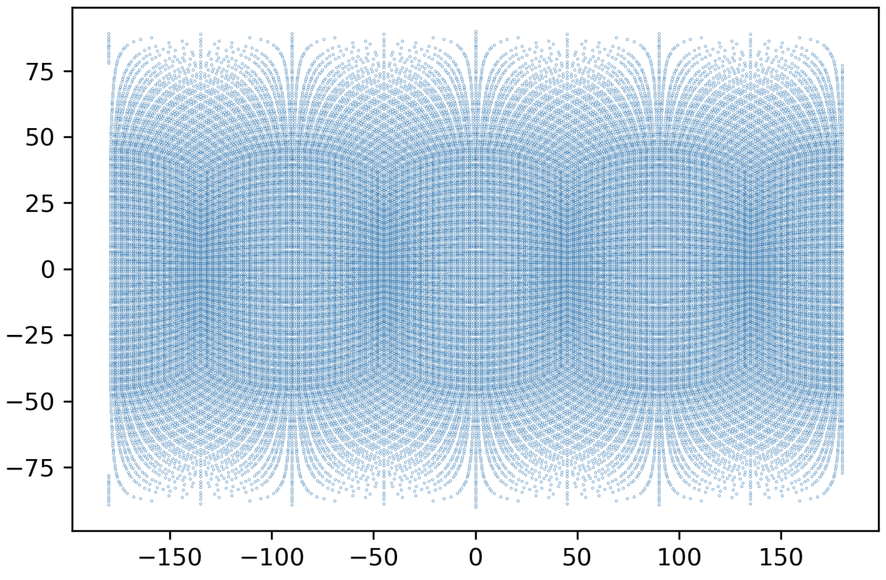
Kevin Paul (Jun 16 2020 at 22:03):There are still some artifacts near the top and bottom borders (little bits of white), but this has to due with the layout of the gridpoints. If you look at the original grid, you can see the gridpoints are symmetric around lon==0, which is where I got the idea:
Screen-Shot-2020-06-16-at-3.51.12-PM.png
Allison Baker (Jun 16 2020 at 22:39):@Kevin Paul That looks good - thanks so much for your help. I will give this a try!
Last updated: May 16 2025 at 17:14 UTC