![]()
Dask Schedulers#
ESDS dask tutorial | 06 February, 2023
Negin Sobhani, Brian Vanderwende, Deepak Cherian, Ben Kirk
Computational & Information Systems Lab (CISL)
negins@ucar.edu, vanderwb@ucar.edu
In this tutorial, you learn:#
Components of Dask Schedulers
Types of Dask Schedulers
Single Machine Schedulers
Related Documentation
Introduction#
As we mentioned in our Dask overview, Dask is composed of two main parts:
Dask Collections (APIs)
Dynamic Task Scheduling
So far, we have talked about different Dask collections, but in this tutorial we are going to talk more about the second part.
The Dask scheduler - our task orchestrator#
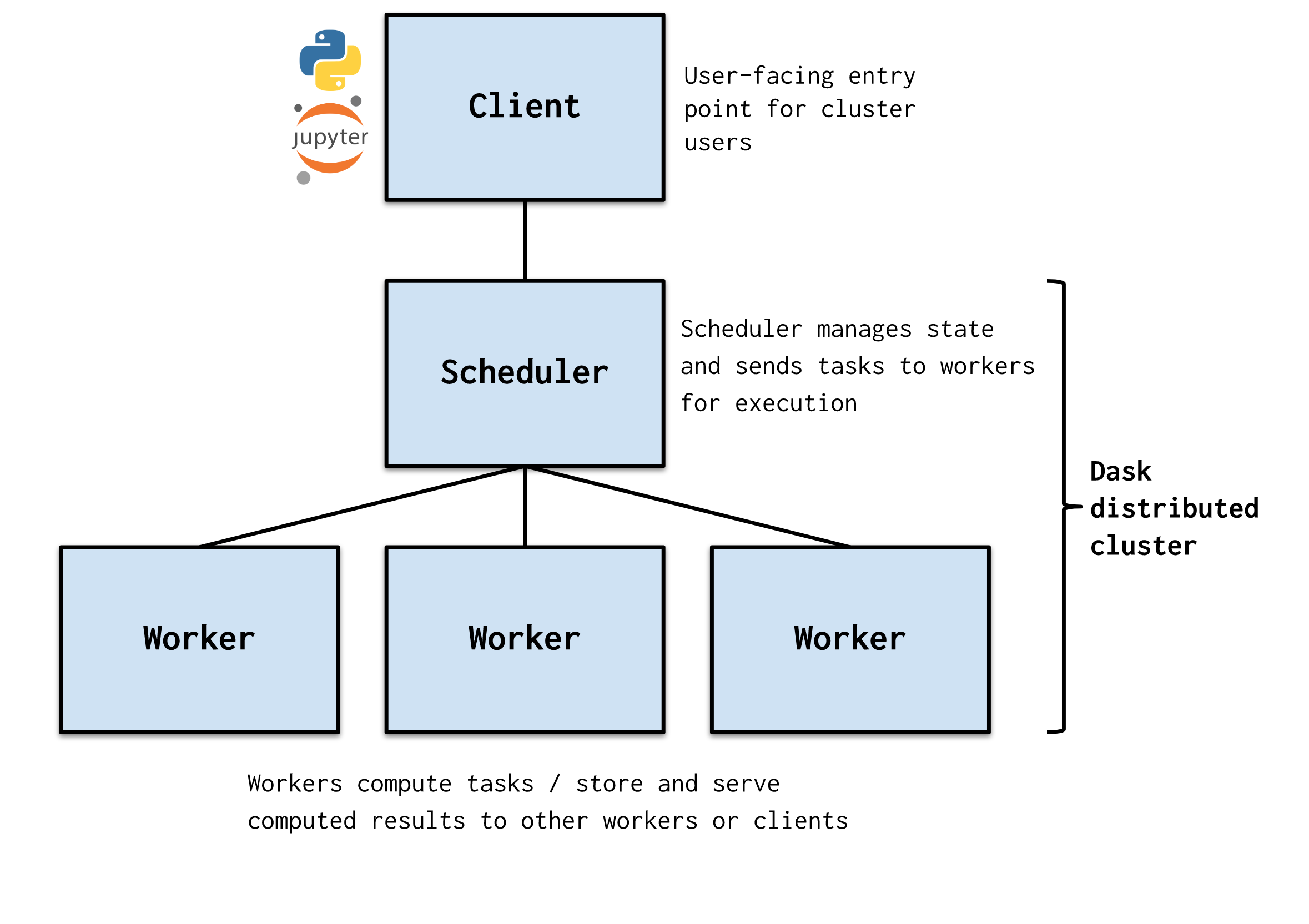
The Dask.distributed task scheduler is a centralized, dynamic system that coordinates the efforts of various dask worker processes spread accross different machines.
When a computational task is submitted, the Dask distributed scheduler sends it off to a Dask cluster - simply a collection of Dask workers. A worker is typically a separate Python process on either the local host or a remote machine.
worker - a Python interpretor which will perform work on a subset of our dataset.
cluster - an object containing instructions for starting and talking to workers.
scheduler - sends tasks from our task graph to workers.
client - a local object that points to the scheduler (often local but not always).
Schedulers#
Dask essentially offers two types of schedulers:

1. Single machine scheduler#
The Single-machine Scheduler schedules tasks and manages the execution of those tasks on the same machine where the scheduler is running.
It is designed to be used in situations where the amount of data or the computational requirements are too large for a single process to handle, but not large enough to warrant the use of a cluster of machines.
It is relatively simple and cheap to use but it does not scale as it only runs on a single machine.
Single machine scheduler is the default choice used by Dask.
In Dask, there are several types of single machine schedulers that can be used to schedule computations on a single machine:
1.1. Single-threaded scheduler#
This scheduler runs all tasks serially on a single thread.
This is only useful for debugging and profiling, but does not have any parallelization.
1.2. Threaded scheduler#
The threaded scheduler uses a pool of local threads to execute tasks concurrently.
This is the default scheduler for Dask, and is suitable for most use cases on a single machine. Multithreading works well for Dask Array and Dask DataFrame.
To select one of the above scheduler for your computation, you can specify it when doing .compute():
For example:
this.compute(scheduler="single-threaded") # for debugging and profiling only
As mentioned above the threaded scheduler is the default scheduler in Dask. But you can set the default scheduler to Single-threaded or multi-processing by:
import dask
dask.config.set(scheduler='synchronous')  # overwrite default with single-threaded scheduler
Multi-processing works well for pure Python code - delayed functions and operations on Dask Bags.
Let’s compare the performance of each of these single-machine schedulers:
Distributed Clusters#
import numpy as np
import dask.array as da
%%time
## - numpy performance
xn = np.random.normal(10, 0.1, size=(20_000, 20_000))
yn = xn.mean(axis=0)
yn
CPU times: user 14.9 s, sys: 1.32 s, total: 16.2 s
Wall time: 16.1 s
array([ 9.99987393,  9.99942047, 10.00069322, ...,  9.99997333,
        9.99945909, 10.00094973])
%%time
# -- dask array using the default
xd = da.random.normal(10, 0.1, size=(20_000, 20_000), chunks=(2000, 2000))
yd = xd.mean(axis=0)
yd.compute()
CPU times: user 14.8 s, sys: 112 ms, total: 14.9 s
Wall time: 3.83 s
array([ 9.99928454,  9.99968075, 10.00027327, ..., 10.00030439,
        9.9999113 ,  9.99947802])
import time
# -- dask testing different schedulers:
for sch in ['threading', 'processes', 'sync']:
    t0 = time.time()
    r = yd.compute(scheduler=sch)
    t1 = time.time()
    print(f"{sch:>10} :  {t1 - t0:0.4f} s")
 threading :  3.7886 s
 processes :  5.2656 s
      sync :  14.7481 s
yd.dask
HighLevelGraph
HighLevelGraph with 4 layers and 240 keys from all layers.
Layer1: normal
normal-6ad96170c4c61710dbc18b74e58c3cb2
|
Layer2: mean_chunk
mean_chunk-1ccb39e699989873e56e0c577ab50469
|
Layer3: mean_combine-partial
mean_combine-partial-9d7408b2918b12ded83c71dd3ff57f3e
|
Layer4: mean_agg-aggregate
mean_agg-aggregate-8bc993aec3b4d7a1fc433f965f460473
|
yd
|
Notice how
syncscheduler takes almost the same time as pure NumPy code.Why is the multiprocessing scheduler so much slower?
If you use the multiprocessing backend, all communication between processes still needs to pass through the main process because processes are isolated from other processes. This introduces a large overhead.
The Dask developers recommend using the Dask Distributed Scheduler which we will cover now.
2. Distributed scheduler#
The Distributed scheduler or
dask.distributedschedules tasks and manages the execution of those tasks on workers from a single or multiple machines.This scheduler is more sophisticated and offers more features including a live diagnostic dashboard which provides live insight on performance and progress of the calculations.
In most cases, dask.distributed is preferred since it is very scalable, and provides and informative interactive dashboard and access to more complex Dask collections such as futures.
2.1. Local Cluster#
A Dask Local Cluster refers to a group of worker processes that run on a single machine and are managed by a single Dask scheduler.
This is useful for situations where the computational requirements are not large enough to warrant the use of a full cluster of separate machines. It provides an easy way to run parallel computations on a single machine, without the need for complex cluster management or other infrastructure.
Let’s start by creating a Local Cluster#
For this we need to set up a LocalCluster using dask.distributed and connect a client to it.
from dask.distributed import LocalCluster, Client

cluster = LocalCluster()
client = Client(cluster)
client
Client
Client-528e046a-a5a4-11ed-928c-3cecef1b11fa
| Connection method: Cluster object | Cluster type: distributed.LocalCluster |
| Dashboard: https://jupyterhub.hpc.ucar.edu/stable/user/negins/casper_16_4/proxy/8787/status |
Cluster Info
LocalCluster
ecdf1399
| Dashboard: https://jupyterhub.hpc.ucar.edu/stable/user/negins/casper_16_4/proxy/8787/status | Workers: 4 |
| Total threads: 4 | Total memory: 16.00 GiB |
| Status: running | Using processes: True |
Scheduler Info
Scheduler
Scheduler-680550a6-4f52-4d2d-99d6-6adbb921c7c9
| Comm: tcp://127.0.0.1:46436 | Workers: 4 |
| Dashboard: https://jupyterhub.hpc.ucar.edu/stable/user/negins/casper_16_4/proxy/8787/status | Total threads: 4 |
| Started: Just now | Total memory: 16.00 GiB |
Workers
Worker: 0
| Comm: tcp://127.0.0.1:45124 | Total threads: 1 |
| Dashboard: https://jupyterhub.hpc.ucar.edu/stable/user/negins/casper_16_4/proxy/39912/status | Memory: 4.00 GiB |
| Nanny: tcp://127.0.0.1:42313 | |
| Local directory: /glade/scratch/negins/dask-worker-space/worker-qsda33zu | |
Worker: 1
| Comm: tcp://127.0.0.1:38609 | Total threads: 1 |
| Dashboard: https://jupyterhub.hpc.ucar.edu/stable/user/negins/casper_16_4/proxy/42328/status | Memory: 4.00 GiB |
| Nanny: tcp://127.0.0.1:41562 | |
| Local directory: /glade/scratch/negins/dask-worker-space/worker-cpl_hk52 | |
Worker: 2
| Comm: tcp://127.0.0.1:43616 | Total threads: 1 |
| Dashboard: https://jupyterhub.hpc.ucar.edu/stable/user/negins/casper_16_4/proxy/44797/status | Memory: 4.00 GiB |
| Nanny: tcp://127.0.0.1:40001 | |
| Local directory: /glade/scratch/negins/dask-worker-space/worker-qnoend2w | |
Worker: 3
| Comm: tcp://127.0.0.1:40873 | Total threads: 1 |
| Dashboard: https://jupyterhub.hpc.ucar.edu/stable/user/negins/casper_16_4/proxy/40512/status | Memory: 4.00 GiB |
| Nanny: tcp://127.0.0.1:36033 | |
| Local directory: /glade/scratch/negins/dask-worker-space/worker-0sqdrcdn | |
☝️ Click the Dashboard link above.
👈 Or click the “Search” 🔍 button in the dask-labextension dashboard.
If no arguments are specified in LocalCluster it will automatically detect the number of CPU cores your system has and the amount of memory and create workers to appropriately fill that.
A LocalCluster will use the full resources of the current JupyterLab session. For example, if you used NCAR JupyterHub, it will use the number of CPUs selected.
Note that LocalCluster() takes a lot of optional arguments, allowing you to configure the number of processes/threads, memory limits and other settings.
You can also find your cluster dashboard link using :
cluster.dashboard_link
'https://jupyterhub.hpc.ucar.edu/stable/user/negins/casper_16_4/proxy/8787/status'
%%time
# -- dask array using the default
xd = da.random.normal(10, 0.1, size=(30_000, 30_000), chunks=(3000, 3000))
yd = xd.mean(axis=0)
yd.compute()
CPU times: user 499 ms, sys: 142 ms, total: 641 ms
Wall time: 10.1 s
array([10.00024901, 10.00025024, 10.00001342, ..., 10.00006029,
        9.99957823, 10.00021491])
Always remember to close your local Dask cluster:
client.shutdown()
Dask Distributed (Cluster)#
So far we have talked about running a job on a local machine.
Dask can be deployed on distributed infrastructure, such as a an HPC system or a cloud computing system.
Dask Clusters have different names corresponding to different computing environments. Some examples are dask-jobqueue for your HPC systems (including PBSCluster) or Kubernetes Cluster for machines on the Cloud.
In section 5, we will talk more about Dask on HPC Systems.