DART-CAM6 reanalysis diagnostic plots

# Imports
import intake
import numpy as np
import pandas as pd
import xarray as xr
import seaborn as sns
import re
import os
import matplotlib.pyplot as plt

import fsspec.implementations.http as fshttp
from pelicanfs.core import PelicanFileSystem, PelicanMap, OSDFFileSystem 

import dask 
from dask_jobqueue import PBSCluster
from dask.distributed import Client
from dask.distributed import performance_report

init_year0  = '1991'
init_year1  = '2020'
final_year0 = '2071'
final_year1 = '2100'

# Set up your scratch folder path
username       = os.environ["USER"]
glade_scratch  = "/glade/derecho/scratch/" + username
print(glade_scratch)

# catalog_url = 'https://osdf-data.gdex.ucar.edu/ncar-gdex/d345001/catalogs/d345001-osdf-zarr.json'
catalog_url = 'https://stratus.gdex.ucar.edu/d345001/catalogs/d345001-https-zarr.json' #NCAR's Object store
print(catalog_url)

# Create a PBS cluster object
cluster = PBSCluster(
    job_name = 'dask-wk24-hpc',
    cores = 1,
    memory = '8GiB',
    processes = 1,
    local_directory = glade_scratch+'/dask/spill',
    log_directory = glade_scratch + '/dask/logs/',
    resource_spec = 'select=1:ncpus=1:mem=8GB',
    queue = 'casper',
    walltime = '5:00:00',
    #interface = 'ib0'
    interface = 'ext'
)

# Create the client to load the Dashboard
client = Client(cluster)
n_workers = 8
cluster.scale(n_workers)
client.wait_for_workers(n_workers = n_workers)
cluster

col = intake.open_esm_datastore(catalog_url)
col

data_var = 'PS'

col_subset = col.search(variable=data_var)
col_subset

col_subset.df['path'].values

col_subset.df

dsets = col_subset.to_dataset_dict(zarr_kwargs={"consolidated": True})
print(f"\nDataset dictionary keys:\n {dsets.keys()}")

# Load the first dataset and display a summary.
dataset_key = list(dsets.keys())[0]
ds = dsets[dataset_key]
ds

# Load the first dataset and display a summary.
dataset_key = list(dsets.keys())[0]
store_name = dataset_key + ".zarr"

ds = dsets[dataset_key]
ds

def getSlice(ds, data_var):
    '''If the data has vertical levels, choose the level closest
       to the Earth's surface for 2-D diagnostic plots.
    '''
    data_slice = ds[data_var]

    if 'lev' in data_slice.dims:
        lastLevel = ds.lev.values[-1]
        data_slice = data_slice.sel(lev = lastLevel)
        data_slice = data_slice.squeeze()

    return data_slice

def getSpatialDimensionNames(data_slice):
    '''Get the spatial dimension names for this data slice.
    '''
    # Determine lat/lon conventions for this slice.
    lat_dim = 'lat' if 'lat' in data_slice.dims else 'slat'
    lon_dim = 'lon' if 'lon' in data_slice.dims else 'slon'
    
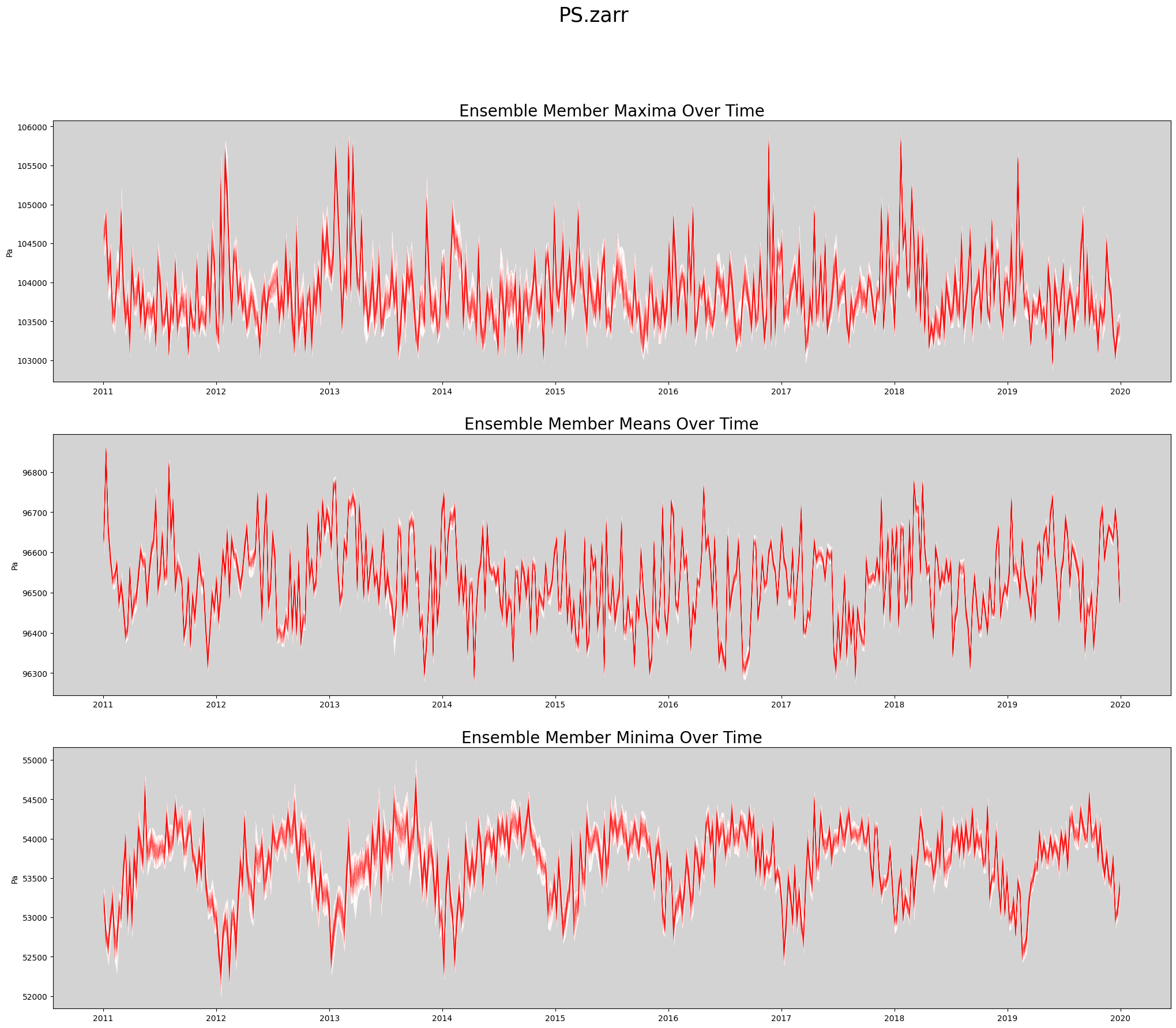
    return [lat_dim, lon_dim]

def plot_timeseries(ds, data_var, store_name):
    '''Create a spaghetti plot for a given variable.
    '''
    figWidth = 25 
    figHeight = 20
    linewidth = 0.5

    numPlotsPerPage = 3
    numPlotCols = 1
    
    # Plot the aggregate statistics across time.
    fig, axs = plt.subplots(3, 1, figsize=(figWidth, figHeight))

    data_slice = getSlice(ds, data_var)
    spatial_dims = getSpatialDimensionNames(data_slice)

    unit_string = ds[data_var].attrs['units']

    # Persist the slice so it's read from disk only once.
    # This is faster when data values are reused many times.
    data_slice = data_slice.persist()

    max_vals = data_slice.max(dim = spatial_dims).transpose()
    mean_vals = data_slice.mean(dim = spatial_dims).transpose()
    min_vals = data_slice.min(dim = spatial_dims).transpose()

    
    rangeMaxs = max_vals.max(dim = 'member_id')
    rangeMins = max_vals.min(dim = 'member_id')
    axs[0].set_facecolor('lightgrey')
    axs[0].fill_between(ds.time, rangeMins, rangeMaxs, linewidth=linewidth, color='white')
    axs[0].plot(ds.time, max_vals, linewidth=linewidth, color='red', alpha=0.1)
    axs[0].set_title('Ensemble Member Maxima Over Time', fontsize=20)
    axs[0].set_ylabel(unit_string)

    rangeMaxs = mean_vals.max(dim = 'member_id')
    rangeMins = mean_vals.min(dim = 'member_id')
    axs[1].set_facecolor('lightgrey')
    axs[1].fill_between(ds.time, rangeMins, rangeMaxs, linewidth=linewidth, color='white')
    axs[1].plot(ds.time, mean_vals, linewidth=linewidth, color='red', alpha=0.1)
    axs[1].set_title('Ensemble Member Means Over Time', fontsize=20)
    axs[1].set_ylabel(unit_string)

    rangeMaxs = min_vals.max(dim = 'member_id')
    rangeMins = min_vals.min(dim = 'member_id')
    axs[2].set_facecolor('lightgrey')
    axs[2].fill_between(ds.time, rangeMins, rangeMaxs, linewidth=linewidth, color='white')
    axs[2].plot(ds.time, min_vals, linewidth=linewidth, color='red', alpha=0.1)
    axs[2].set_title('Ensemble Member Minima Over Time', fontsize=20)
    axs[2].set_ylabel(unit_string)

    plt.suptitle(store_name, fontsize=25)
    
    return fig

%%time

store_name = f'{data_var}.zarr'
fig = plot_timeseries(ds, data_var, store_name)

cluster.close()