Nino indices from HadISST data

# Import
import intake
import numpy as np
import xarray as xr
import nc_time_axis
import os
import matplotlib.pyplot as plt

import dask 
from dask_jobqueue import PBSCluster
from dask.distributed import Client
from dask.distributed import performance_report

# Set up your sratch folder path
username       = os.environ["USER"]
glade_scratch  = "/glade/derecho/scratch/" + username
print(glade_scratch)

#### Useful function ###
def area_mean(da):
    """
    Area-weighted mean over lat/lon using cos(lat) weighting.
    Assumes da has dims including lat, lon.
    """
    weights = np.cos(np.deg2rad(da["latitude"]))
    weights.name = "weights"
    return da.weighted(weights).mean(dim=("latitude", "longitude"), skipna=True)

def lon_to_360(da):
    """Ensure longitude is [0, 360) and sorted.""" 
    lon_name = "lon" if "lon" in da.coords else "longitude"
    lon = da[lon_name]
    lon360 = (lon % 360)   
    #The above logic is tricky for negative divisors or dividends and is not guaranteed to work in other programming languages
    #For more details, see https://en.wikipedia.org/wiki/Modulo
    da = da.assign_coords({lon_name: lon360}).sortby(lon_name)
    return da

##
def nino_index_series(sst, region):
    lat0, lat1 = region["latitude"]
    lon0, lon1 = region["longitude"]
    sub = sst.sel(latitude=slice(lat0, lat1), longitude=slice(lon0, lon1))
    return area_mean(sub)

# Create a PBS cluster object
cluster = PBSCluster(
    job_name = 'dask-wk25',
    cores = 1,
    memory = '8GiB',
    processes = 1,
    local_directory = glade_scratch+'/dask/spill/',
    log_directory = glade_scratch + '/dask/logs/',
    resource_spec = 'select=1:ncpus=1:mem=8GB',
    queue = 'casper',
    walltime = '5:00:00',
    interface = 'ext'
)

# Create the client to load the Dashboard
client = Client(cluster)

n_workers = 5
cluster.scale(n_workers)
client.wait_for_workers(n_workers = n_workers)
cluster

import gzip
import tempfile

with gzip.open("/gdex/data/d277003/HadISST_sst.nc.gz", "rb") as f:
    raw = f.read()

with tempfile.NamedTemporaryFile(suffix=".nc") as tmp:
    tmp.write(raw)
    tmp.flush()
    ds = xr.open_dataset(tmp.name)

sst_raw = ds.sst
sst_raw

sst = lon_to_360(sst_raw)
sst

NINO_REGIONS = {
    "nino12": {"latitude": (0, -10),  "longitude": (270, 280)},  # 90W–80W
    "nino3":  {"latitude": (5, -5),   "longitude": (210, 270)},  # 150W–90W
    "nino34": {"latitude": (5, -5),   "longitude": (190, 240)},  # 170W–120W
    "nino4":  {"latitude": (5, -5),   "longitude": (160, 210)},  # 160E–150W
}

nino_raw = xr.Dataset({name: nino_index_series(sst, reg) for name, reg in NINO_REGIONS.items()})
nino_raw

nino_raw.to_dataframe().plot(subplots=True, figsize=(10, 8), lw=1)
plt.gcf().supylabel(r'SST ($^\circ$ C)')
plt.gcf().supxlabel('time')
plt.tight_layout()
plt.gcf().suptitle(' Nino indices from monthly HadISST data',fontsize=12,fontweight='bold',y=0.999)
plt.show()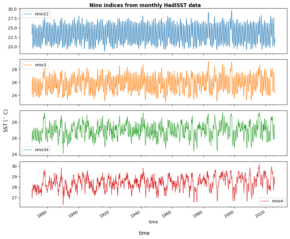

# %%time
# sst = xr.open_dataset('/gdex/data/d277003/HadISST_sst.nc.gz',engine='netcdf4')

cluster.close()