NCAR S-Pol Radar moments data

Required Packages¶

Please ensure the following packages are installed before proceeding.

Category	Package	Purpose
Data Access & Analysis	`zarr` > v3.1.5	Read/write Zarr format data stores
	`xarray` > v2015.7.1	Lazy loading and array manipulation
Radar Analysis	`xradar`	Read and process radar data
	`arm-pyart`	ARM radar analysis toolkit
Visualization	`matplotlib`	General-purpose plotting
	`cartopy`	Geospatial map projections
	`cmweather`	Colormaps tailored for weather data

Step 1 - Visualize the Radar data¶

The dataset contains two types of files corresponding to two different S‑Pol scanning strategies: Range–Height Indicator (RHI) and Plan Position Indicator (PPI). In this example, our goal is to quickly plot both types of radar scans and, if desired, combine multiple scans to perform cross‑file analysis.

Step 2 - Locate the Dataset¶

The dataset is freely available on the NCAR GDEX portal and is stored on NCAR’s BOREAS object storage. This notebook demonstrates two access methods:

NCAR HPC — direct BOREAS access for users on NCAR’s HPC systems
Remote — internet-based access for users outside of NCAR

# Please specify your preferred data access method: the Data URL or the GDEX POSIX path. 
# We are also open to suggestions for the most useful access method for our target users.
hpc_url_horizontal_scan = "https://boreas.hpc.ucar.edu:6443/gdex-data/d694517/v2.0_zarr/cfrad.20220525_030910.927_to_20220525_031137.777_SPOL_PrecipSur2_SUR.zarr"
remote_url_vertical_scan = "https://osdf-director.osg-htc.org/ncar-gdex/d694517/v2.0_zarr/cfrad.20220525_015443.665_to_20220525_015709.985_SPOL_PrecipRhi2_RHI.zarr"

Step 3 - Open the Data¶

Radar data in Zarr format is best opened with xr.open_datatree rather than the standard xr.open_dataset. This is because the data follows the CfRadial2 convention, which organizes radar sweeps into a hierarchical tree structure — all sweeps from a single scan are stored together in one Zarr store, with each sweep as a separate node in the tree.

For background on the CfRadial2 format and how sweep data is structured, see this article provided by EarthMover: From Files to Datasets: FM-301 and the Future of Radar Interoperability

import xarray as xr
dt_horizontal = xr.open_datatree(hpc_url_horizontal_scan, engine="zarr", decode_timedelta=False)
dt_vertical = xr.open_datatree(remote_url_vertical_scan, engine="zarr", decode_timedelta=False)

dt_horizontal

Loading...

dt_vertical

Loading...

Step 4 - Focus on a Single Sweep¶

A DataTree returned by xr.open_datatree contains multiple nodes, each corresponding to one radar sweep (e.g., sweep_0, sweep_1, ...). To visualize or analyze the data, we first extract a single sweep as a standard xarray.Dataset using node indexing.

Each sweep node contains the full set of radar variables (e.g., reflectivity, velocity, differential reflectivity) along with the associated coordinates (range, azimuth or elevation, and time) for that scan.

ds_vertical_sweep0 = dt_vertical["sweep_0"].to_dataset()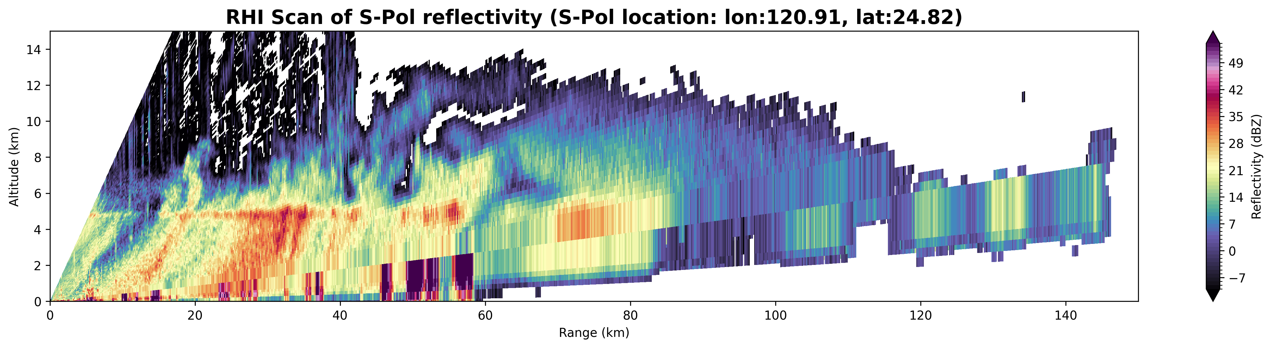
ds_vertical_sweep0

Loading...

Step 5 - Visualize the RHI Scan¶

With the vertical sweep extracted, we now prepare and plot the Range-Height Indicator (RHI) scan. The following three cells:

Define a helper function — computes the altitude (in km) of each radar gate from its range and elevation angle, accounting for Earth’s curvature.
Preprocess the sweep — applies the altitude function to add rhi_alt as a new coordinate, converts range from meters to kilometers, and updates variable attributes.
Plot the reflectivity (DBZ) — renders a 2D pcolormesh of reflectivity as a function of range and altitude using the ChaseSpectral colormap from cmweather.

import numpy as np
# calculate RHI altitude from range and elevation angle
def calculate_rhi_altitude(r,e):
    """Calculate radar beam altitude (kilometers) from range (meters) and elevation angle (radians).
    """
    rEarth = 6371000.0  # meters
    e_deg = np.deg2rad(e)
    return (np.sqrt(r**2 + rEarth**2 + 2*r*rEarth*np.sin(e_deg)) - rEarth) / 1000.0  # output in km

# calculate RHI altitude
da_rhi_alt = calculate_rhi_altitude(ds_vertical_sweep0['range'], ds_vertical_sweep0['elevation']).compute()

# add RHI altitude as a coordinate
ds_vertical_sweep0['rhi_alt'] = da_rhi_alt
ds_vertical_sweep0 = ds_vertical_sweep0.set_coords('rhi_alt')

# convert range to km
ds_vertical_sweep0['range'] = ds_vertical_sweep0['range'] / 1000.0  # Convert to km

# update variable attributes
ds_vertical_sweep0['rhi_alt'].attrs = {}
ds_vertical_sweep0['rhi_alt'].attrs['long_name'] = 'RHI Altitude'
ds_vertical_sweep0['rhi_alt'].attrs['units'] = 'kilometers'
ds_vertical_sweep0['range'].attrs['units'] = 'kilometers'

import matplotlib.pyplot as plt
import cmweather # colorblind friendly weather data visualization (https://cmweather.readthedocs.io/)

# plot DBZ with range and RHI altitude
fig, ax = plt.subplots(figsize=(20, 4),dpi=300)
ds_vertical_sweep0.DBZ.plot.pcolormesh(x='range', y='rhi_alt', cmap="ChaseSpectral", levels=np.arange(-10, 55, 1), ax=ax,add_colorbar=False)
ax.set_xlabel("Range (km)")
ax.set_ylabel("Altitude (km)")
ax.set_title(f"RHI Scan of S-Pol reflectivity (S-Pol location: lon:{ds_vertical_sweep0.longitude.values:0.2f}, lat:{ds_vertical_sweep0.latitude.values:0.2f})", fontsize=16, fontweight='bold')
ax.set_ylim(0,15)
ax.set_xlim(0,150)
plt.colorbar(ax.collections[0], ax=ax, label="Reflectivity (dBZ)")

Step 6 - Visualize the PPI Scan¶

This step visualizes the horizontal Plan Position Indicator (PPI) surveillance scan using xradar georeferencing utilities. The following three cells:

Georeference the DataTree — uses xradar.georeference to compute Cartesian x, y, z coordinates from the radar’s polar coordinates (range, azimuth, elevation), then extracts sweep_0 as a Dataset.
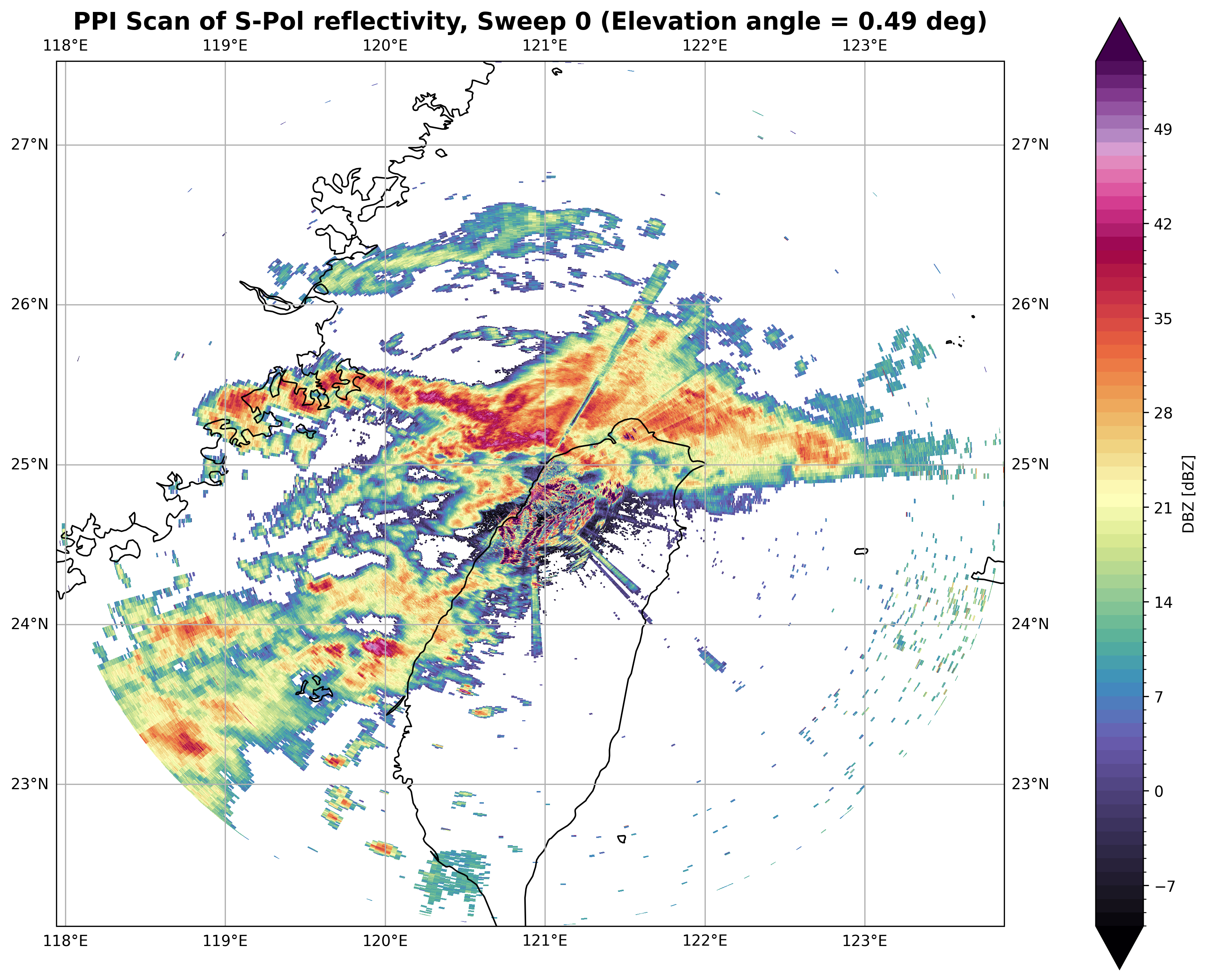
Plot in Cartesian coordinates — renders the reflectivity field on a flat x/y grid (distance east vs. distance north in meters) using matplotlib.
Plot on a geographic map — reprojects the same reflectivity field onto a cartopy map with coastlines and gridlines, providing a geospatial context for the radar coverage area.

import xradar as xd

### Utilize the xradar georeference utilities to get the x, y, z coordinates for the horizontal scan data.
dt_horizontal = dt_horizontal.xradar.georeference()
dt_horizontal = xd.georeference.get_x_y_z_tree(dt_horizontal)
ds_sweep_0 = dt_horizontal["sweep_0"].to_dataset()
da_dbz = ds_sweep_0["DBZ"]

#plot reflectivity field on a flat x/y grid 
fig, ax = plt.subplots(figsize=(12, 12),dpi=300)
pcm = da_dbz.plot(
    ax=ax,
    x="x",
    y="y",
    cmap="ChaseSpectral", 
    levels=np.arange(-10, 55, 1), 
    add_colorbar=True,
    cbar_kwargs={
        "label": "Reflectivity (dBZ)",
        "shrink": 0.8,
        "pad": 0.02
    }
)
ax.set_title(f"PPI Scan (Sweep 0) of S-Pol reflectivity (S-Pol location: lon:{da_dbz.longitude.values:0.2f}, lat:{da_dbz.latitude.values:0.2f})", fontsize=16, fontweight='bold')
ax.set_xlabel("Distance East (m)", fontsize=12)
ax.set_ylabel("Distance North (m)", fontsize=12)
ax.set_aspect("equal")  
ax.grid(False)
plt.tight_layout()
plt.show()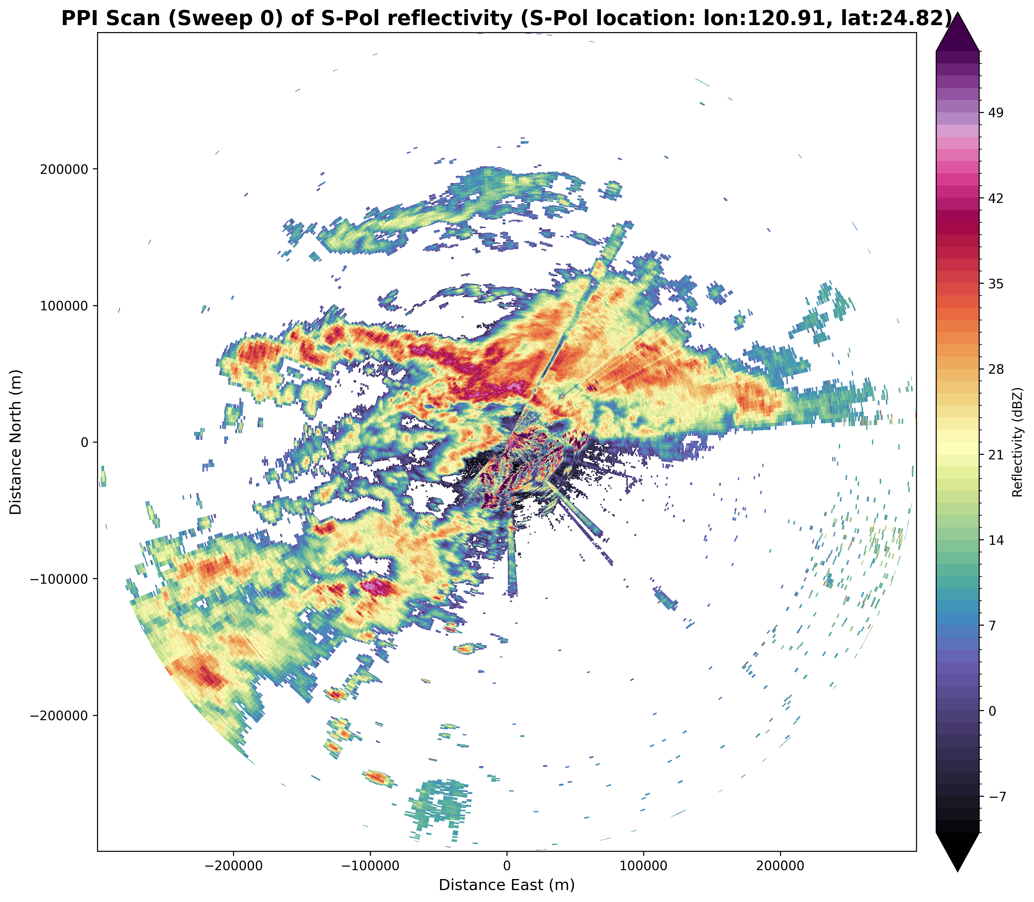

import cartopy
#Plot on geographic map
proj_crs = xd.georeference.get_crs(ds_sweep_0)
cart_crs = cartopy.crs.Projection(proj_crs)

fig = plt.figure(figsize=(12, 12), dpi=300)
ax = fig.add_subplot(111, projection=cartopy.crs.PlateCarree())
da_dbz.plot(
    x="x",
    y="y",
    cmap="ChaseSpectral", 
    levels=np.arange(-10, 55, 1), 
    transform=cart_crs,
    cbar_kwargs=dict(pad=0.075, shrink=0.75),
)
ax.coastlines()
ax.gridlines(draw_labels=True)
ax.set_title(f"PPI Scan of S-Pol reflectivity, Sweep 0 (Elevation angle = {ds_sweep_0.elevation.values[0]:0.2f} deg)", fontsize=16, fontweight='bold')
ax.set_aspect("equal")  
ax.grid(False)
plt.tight_layout()
plt.show()

/glade/u/home/chiaweih/test_xradar/.venv/lib/python3.11/site-packages/cartopy/mpl/geoaxes.py:1762: UserWarning: The input coordinates to pcolormesh are interpreted as cell centers, but are not monotonically increasing or decreasing. This may lead to incorrectly calculated cell edges, in which case, please supply explicit cell edges to pcolormesh.
  result = super().pcolormesh(*args, **kwargs)

Access Prediction of Rainfall Extremes Campaign In the Pacific (PRECIP) field campaign radar data¶

Required Packages¶

Step 1 - Visualize the Radar data¶

Step 2 - Locate the Dataset¶

Step 3 - Open the Data¶

Step 4 - Focus on a Single Sweep¶

Step 5 - Visualize the RHI Scan¶

Step 6 - Visualize the PPI Scan¶