Required Packages
Here we will list the required packages to be able to perform the following steps. Please make sure to installed the packages before moving forward
intakeintake-esm >= 2025.12.12matplotlibxarraykerchunk
Step 1 - know what you want
In this example, we will show how to find the needed variables in the JRA3Q data. Let’s start by assuming we need to find the surface temperature in the dataset. For the analysis, we will plot a spatial map of surface temperature and calculate the global mean surface temperature over the entire period of the dataset.
Step 2 - Locate the Catalog
On the NCAR GDEX portal, go to the Data Access tab for your selected dataset. Scroll down to find a purple row labeled Catalog with an Analysis ready tag. Click on the Web File List to view the available catalog files in .json format. Use the copy Full URL button to obtain the direct link to the catalog file, which you can use in your analysis workflow.

(a)Click on Data Acess Button
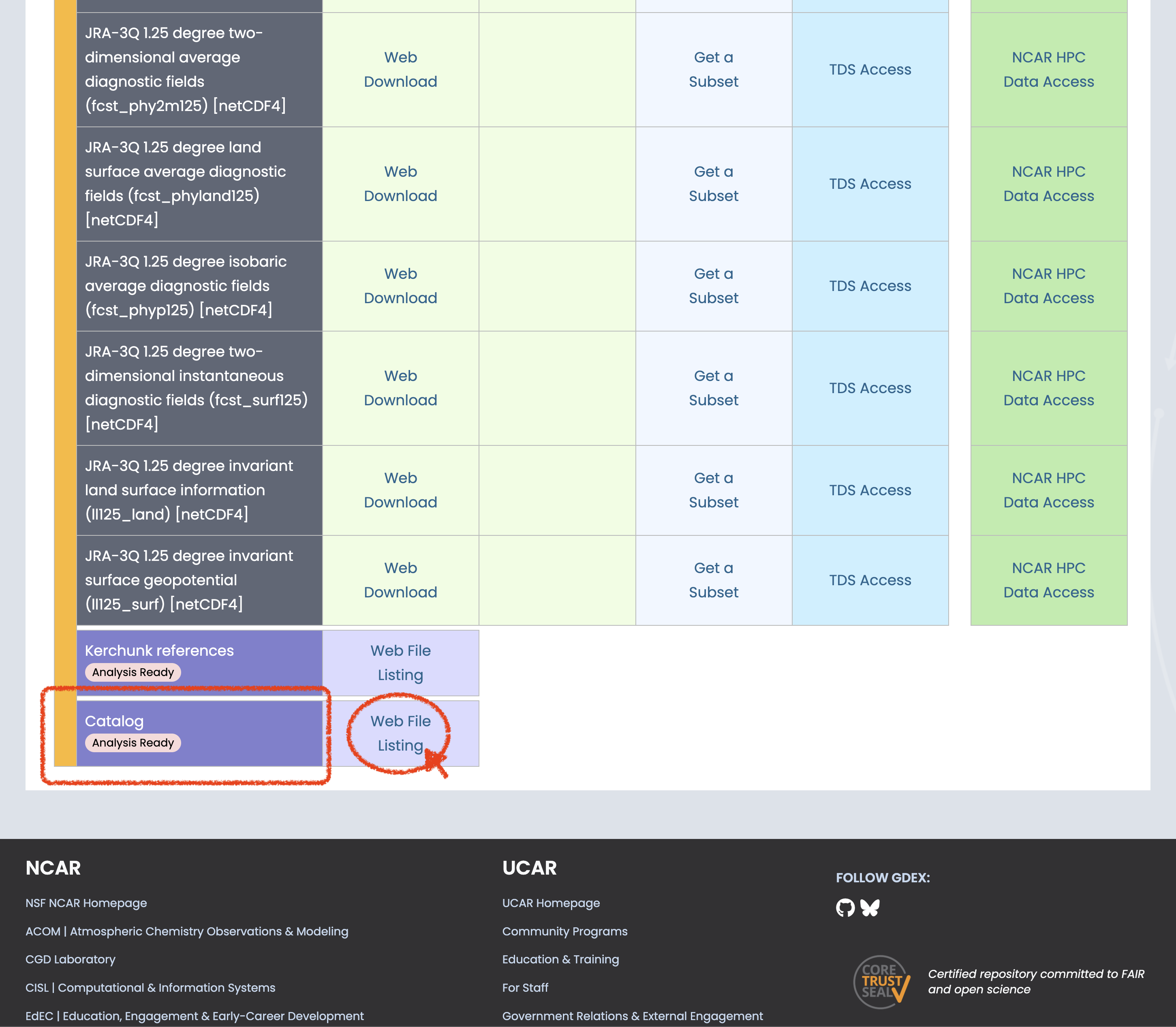
(b)Scroll to bottom to find the Catalog of AI Ready and click on the web file listing

(c)Pick one refence file URL that suits you
Figure 1:Steps to Find the AI Ready Catalog!
Step 3 - Open the Catalog (remote https access)
This is the steps where the intake and intake-esm package works their magic to show us all the data that have been cataloged without the need of actually knowing the data/folder structure that is used in the background.
# Catalog location for NCAR GDEX AI Ready Format datasets
catalog_url = "https://data.gdex.ucar.edu/d640000/catalogs/d640000-https.json"
import intake
cat = intake.open_esm_datastore(catalog_url)# take a look at the first 15 rows of the catalog
cat.df.head(5)Step 4 - Refine the Search
Here is where we can use the intake esm to filter the search and try to find the surface temperature variables we need.
# List all the long name in the catalog
cat.df['long_name'].values.tolist()[:5]  # show first 5 long names
['Square of Brunt-Vaisala frequency',
'Geopotential height',
'Montgomery stream function',
'original number of grid points per latitude circle',
'Pressure']# Filter the catalog for variables with 'temp' in their long name
cat_filtered = cat.search(long_name='temp*')cat_filtered.df.head(5)Step 5 - Data Analysis
Here we pick to focus on the variable tmp2m-hgt-an-gauss. A quick way to load the data into memory from the catalog is to use the .to_dataset_dict() methods. This load the data into the memory as dictionary.
cat_analysis = cat.search(variable='tmp2m-hgt-an-gauss')
dict_datasets = cat_analysis.to_dataset_dict(xarray_open_kwargs={'engine':'kerchunk'})
--> The keys in the returned dictionary of datasets are constructed as follows:
	'variable.short_name'
# take a look at the dataset loaded
dict_datasets
{'tmp2m-hgt-an-gauss.tmp2m-hgt-an-gauss': <xarray.Dataset> Size: 3TB
Dimensions: (time: 114080,
lat: 480, lon: 960)
Coordinates:
* lat (lat) float64 4kB 89....
* lon (lon) float64 8kB 0.0...
* time (time) datetime64[ns] 913kB ...
Data variables: (12/17)
depr2m-hgt-an-gauss (time, lat, lon) float32 210GB dask.array<chunksize=(1, 480, 960), meta=np.ndarray>
original_number_of_grid_points_per_latitude_circle (time, lat) int32 219MB dask.array<chunksize=(1, 480), meta=np.ndarray>
pot-sfc-an-gauss (time, lat, lon) float32 210GB dask.array<chunksize=(1, 480, 960), meta=np.ndarray>
pres-sfc-an-gauss (time, lat, lon) float32 210GB dask.array<chunksize=(1, 480, 960), meta=np.ndarray>
prmsl-msl-an-gauss (time, lat, lon) float32 210GB dask.array<chunksize=(1, 480, 960), meta=np.ndarray>
rh2m-hgt-an-gauss (time, lat, lon) float32 210GB dask.array<chunksize=(1, 480, 960), meta=np.ndarray>
... ...
ugrd10m-hgt-an-gauss (time, lat, lon) float32 210GB dask.array<chunksize=(1, 480, 960), meta=np.ndarray>
utc_date_int (time) int32 456kB dask.array<chunksize=(1024,), meta=np.ndarray>
utc_date_str (time) object 913kB dask.array<chunksize=(512,), meta=np.ndarray>
vgrd10m-hgt-an-gauss (time, lat, lon) float32 210GB dask.array<chunksize=(1, 480, 960), meta=np.ndarray>
weasd-sfc-an-gauss (time, lat, lon) float32 210GB dask.array<chunksize=(1, 480, 960), meta=np.ndarray>
weight (time, lat) float64 438MB dask.array<chunksize=(1, 480), meta=np.ndarray>
Attributes: (12/102)
jma_data_provider: Japan Meteorological ...
jma_data_provider_url: https://www.jma.go.jp...
jma_data_provider_address: 3-6-9 Toranomon, Mina...
jma_data_provider_email: <jra@met.kishou.go.jp>
jma_data_title: Japanese Reanalysis f...
jma_data_abstract: JMA is currently cond...
... ...
intake_esm_attrs:long_name: 2m temperature
intake_esm_attrs:units: K
intake_esm_attrs:start_time: 1947-09-01 00:00:00
intake_esm_attrs:end_time: 2025-09-30 18:00:00
intake_esm_attrs:frequency: 21600000000000 nanose...
intake_esm_dataset_key: tmp2m-hgt-an-gauss.tm...}# a quick one time slice glance of the data
ds = dict_datasets['tmp2m-hgt-an-gauss.tmp2m-hgt-an-gauss']
ds['tmp2m-hgt-an-gauss'].isel(time=0).plot(cmap='coolwarm')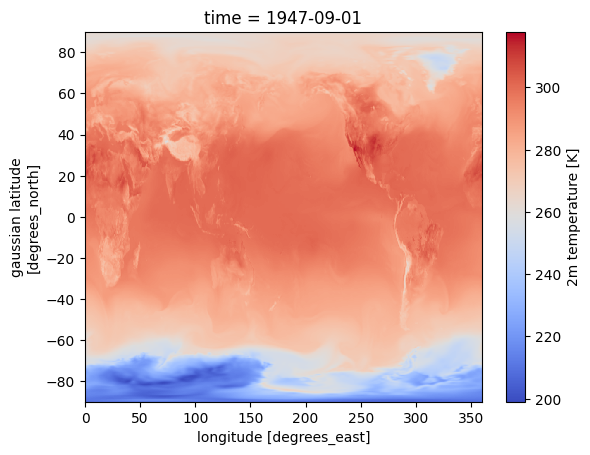
%%time
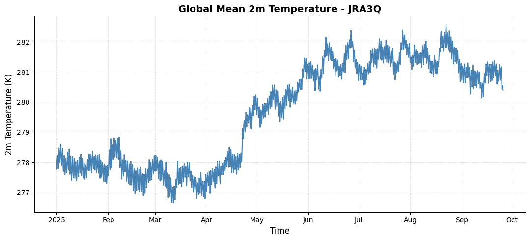
# a quick calculation of global mean surface temperature hourly time series
da_tmp2m = ds['tmp2m-hgt-an-gauss'].sel(time=slice('2025-01-01','2025-09-25')).mean(dim=['lat','lon']).compute()
CPU times: user 1min 53s, sys: 2.56 s, total: 1min 56s
Wall time: 1min 33s
import matplotlib.pyplot as plt

# Create a customized time series plot
fig = plt.figure(figsize=(10, 4))
ax = fig.add_axes([0, 0, 1, 1])

# plot time series
da_tmp2m.plot(ax=ax, color='steelblue', linewidth=1.5)

# Customize the plot
ax.set_title('Global Mean 2m Temperature - JRA3Q', fontsize=14, fontweight='bold')
ax.set_xlabel('Time', fontsize=12)
ax.set_ylabel('2m Temperature (K)', fontsize=12)
ax.grid(True, alpha=0.3, linestyle='--')
ax.spines['top'].set_visible(False)
ax.spines['right'].set_visible(False)
Step 3.1 - Open the Catalog (posix access)
This is the steps where the intake and intake-esm package works their magic to show us all the data that have been cataloged without the need of actually knowing the data/folder structure that is used in the background with POSIX path provided by the GDEX portal for the NCAR HPC user.
# Catalog location for NCAR GDEX AI Ready Format datasets
catalog_path = "/gdex/data/d640000/catalogs/d640000-posix.json"
import intake
cat = intake.open_esm_datastore(catalog_path)# take a look at the first 15 rows of the catalog
cat.df.head(5)Step 4.1 - Refine the Search
Here is where we can use the intake esm to filter the search and try to find the surface temperature variables we need.
# List all the long name in the catalog
cat.df['long_name'].values.tolist()[:5]  # show first 5 long names
['Square of Brunt-Vaisala frequency',
'Geopotential height',
'Montgomery stream function',
'original number of grid points per latitude circle',
'Pressure']# Filter the catalog for variables with 'temp' in their long name
cat_filtered = cat.search(long_name='temp*')cat_filtered.df.head(5)Step 5.1 - Data Analysis
Here we pick to focus on the variable tmp2m-hgt-an-gauss and deliberately choose the same variable to compare the near data calculation to test the computational speed difference. A quick way to load the data into memory from the catalog is to use the .to_dataset_dict() methods. This load the data into the memory as dictionary.
cat_analysis = cat.search(variable='tmp2m-hgt-an-gauss')
dict_datasets = cat_analysis.to_dataset_dict(xarray_open_kwargs={'engine':'zarr'})
--> The keys in the returned dictionary of datasets are constructed as follows:
	'variable.short_name'
# take a look at the dataset loaded
dict_datasets
{'tmp2m-hgt-an-gauss.tmp2m-hgt-an-gauss': <xarray.Dataset> Size: 3TB
Dimensions: (time: 114080,
lat: 480, lon: 960)
Coordinates:
* lat (lat) float64 4kB 89....
* lon (lon) float64 8kB 0.0...
* time (time) datetime64[ns] 913kB ...
Data variables: (12/17)
depr2m-hgt-an-gauss (time, lat, lon) float32 210GB dask.array<chunksize=(1, 480, 960), meta=np.ndarray>
original_number_of_grid_points_per_latitude_circle (time, lat) int32 219MB dask.array<chunksize=(1, 480), meta=np.ndarray>
pot-sfc-an-gauss (time, lat, lon) float32 210GB dask.array<chunksize=(1, 480, 960), meta=np.ndarray>
pres-sfc-an-gauss (time, lat, lon) float32 210GB dask.array<chunksize=(1, 480, 960), meta=np.ndarray>
prmsl-msl-an-gauss (time, lat, lon) float32 210GB dask.array<chunksize=(1, 480, 960), meta=np.ndarray>
rh2m-hgt-an-gauss (time, lat, lon) float32 210GB dask.array<chunksize=(1, 480, 960), meta=np.ndarray>
... ...
ugrd10m-hgt-an-gauss (time, lat, lon) float32 210GB dask.array<chunksize=(1, 480, 960), meta=np.ndarray>
utc_date_int (time) int32 456kB dask.array<chunksize=(1024,), meta=np.ndarray>
utc_date_str (time) object 913kB dask.array<chunksize=(512,), meta=np.ndarray>
vgrd10m-hgt-an-gauss (time, lat, lon) float32 210GB dask.array<chunksize=(1, 480, 960), meta=np.ndarray>
weasd-sfc-an-gauss (time, lat, lon) float32 210GB dask.array<chunksize=(1, 480, 960), meta=np.ndarray>
weight (time, lat) float64 438MB dask.array<chunksize=(1, 480), meta=np.ndarray>
Attributes: (12/102)
jma_data_provider: Japan Meteorological ...
jma_data_provider_url: https://www.jma.go.jp...
jma_data_provider_address: 3-6-9 Toranomon, Mina...
jma_data_provider_email: <jra@met.kishou.go.jp>
jma_data_title: Japanese Reanalysis f...
jma_data_abstract: JMA is currently cond...
... ...
intake_esm_attrs:long_name: 2m temperature
intake_esm_attrs:units: K
intake_esm_attrs:start_time: 1947-09-01 00:00:00
intake_esm_attrs:end_time: 2025-09-30 18:00:00
intake_esm_attrs:frequency: 21600000000000 nanose...
intake_esm_dataset_key: tmp2m-hgt-an-gauss.tm...}%%time
# a quick calculation of global mean surface temperature hourly time series
da_tmp2m = ds['tmp2m-hgt-an-gauss'].sel(time=slice('2025-01-01','2025-09-25')).mean(dim=['lat','lon']).compute()
CPU times: user 1min 58s, sys: 1.97 s, total: 2min
Wall time: 1min 38s
POSIX and HTTPS
This simple test demonstrates the difference between POSIX and remote HTTPS access. Results may vary depending on the timing of the test. In this notebook, we performed two tests at different times: one showed almost no difference in total access time, while the other showed POSIX access to be approximately 30% faster than HTTPS. The kerchunk reference access highlights the potential for remote data streaming to approach the speed of local access. Factors such as network speed and the size of the data subset requested can influence performance. Overall, these results show that using intake-esm with the Dask on the backend provides efficient concurrent requests for data access, even when your workload is not running on the NCAR HPC system.