Mean total precipitation from ERA5

Access ERA5 preciptation data from NCAR GDEX¶

Required Packages¶

Please make sure to installed the packages before moving forward

intake
intake-esm >= 2025.7.9
matplotlib
xarray
dask
kerchunk
cartopy

import matplotlib.pyplot as plt
import numpy as np
import os
import xarray as xr
import intake
import intake_esm
import pandas as pd
import cartopy.crs as ccrs
import cartopy.feature as cfeature
import dask 
from dask_jobqueue import PBSCluster
from dask.distributed import Client

Step 1 - Locate the Dataset¶

On the NCAR GDEX portal, go to the Data Access tab for the ERA5 dataset to find the intake-ESM catalogs needed to access data. In this notebook we will use GDEX POSIX catalog.

# Please specify your preferred data access method: the Data URL or the GDEX POSIX path. 
era5_catalog_posix = '/gdex/data/d633000/catalogs/d633000-posix.json'
# era5_catalog_url = 'http://data.gdex.ucar.edu/d633000/catalogs/d633000-https.json'

Step 2 - Set up cluster¶

# Set up your sratch folder path
username       = os.environ["USER"]
glade_scratch  = "/glade/derecho/scratch/" + username
print(glade_scratch)

/glade/derecho/scratch/harshah

# Create a PBS cluster object
cluster = PBSCluster(
    job_name = 'dask-wk25',
    cores = 1,
    memory = '8GiB',
    processes = 1,
    local_directory = glade_scratch+'/dask/spill/',
    log_directory = glade_scratch + '/dask/logs/',
    resource_spec = 'select=1:ncpus=1:mem=8GB',
    queue = 'casper',
    walltime = '5:00:00',
    interface = 'ext'
)

/glade/u/home/harshah/venvs/osdf/lib/python3.10/site-packages/distributed/node.py:187: UserWarning: Port 8787 is already in use.
Perhaps you already have a cluster running?
Hosting the HTTP server on port 45641 instead
  warnings.warn(

# Create the client to load the Dashboard
client = Client(cluster)

n_workers = 5
cluster.scale(n_workers)
client.wait_for_workers(n_workers = n_workers)
cluster

Step 3 - Open the catalog, find and load the variable of interest¶

%%time
era5_cat = intake.open_esm_datastore(era5_catalog_posix)
era5_cat

CPU times: user 670 μs, sys: 23.4 ms, total: 24 ms
Wall time: 124 ms

era5_cat.df[['variable','long_name']].drop_duplicates()

cat_subset = era5_cat.search(variable='MTPR')
cat_subset.df

%%time
dset_subset = cat_subset.to_dataset_dict()


--> The keys in the returned dictionary of datasets are constructed as follows:
	'variable.short_name'

CPU times: user 938 ms, sys: 147 ms, total: 1.08 s
Wall time: 7.9 s

Step 4 - Data Analysis¶

mtpr = dset_subset['MTPR.mtpr']
mtpr

Plot mean total precipitation for a particular forecast_initial_time and forecast_hour. Let us pick a random forecast hour and day in July, when we expect to see summer precipitation in the Northern hemisphere and tropics

da = mtpr.MTPR.isel(forecast_hour=6).sel(forecast_initial_time='2023-07-15T06:00:00.000000000')

# 2) Make a Cartopy map axis
proj = ccrs.PlateCarree()  
fig, ax = plt.subplots(figsize=(12, 6), subplot_kw={"projection": proj})

# 3) Plot onto that axis
im = da.plot(
    ax=ax,  
    transform=ccrs.PlateCarree(),
    cmap = 'Blues',
    x="longitude",
    y="latitude",
    #robust=True,                
    cbar_kwargs={"label": getattr(da, "units", "")},
)

ax.coastlines(color="black", linewidth=1.0)

<cartopy.mpl.feature_artist.FeatureArtist at 0x14bef36f4400>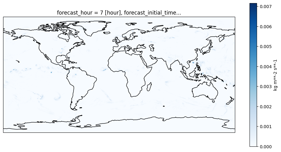

# Close the cluster
cluster.close()