
Calculating Climatologies#
Overview#
Calculating climatologies in Python is a common task in geoscience workflows. This notebook will cover:
Example Data#
The dataset used in this notebook originated from the Community Earth System Model v2 (CESM2), and is retrieved from the Pythia-datasets repository
The dataset contains 15 years of monthly mean sea surface temperatures (TOS) from January 2000 to December 2014
from pythia_datasets import DATASETS
import xarray as xr

# Get data
filepath = DATASETS.fetch("CESM2_sst_data.nc")
ds = xr.open_dataset(filepath)

ds
Downloading file 'CESM2_sst_data.nc' from 'https://github.com/ProjectPythia/pythia-datasets/raw/main/data/CESM2_sst_data.nc' to '/home/runner/.cache/pythia-datasets'.
/home/runner/micromamba/envs/geocat-applications/lib/python3.12/site-packages/xarray/conventions.py:286: SerializationWarning: variable 'tos' has multiple fill values {1e+20, 1e+20} defined, decoding all values to NaN.
  var = coder.decode(var, name=name)
<xarray.Dataset> Size: 47MB
Dimensions:    (time: 180, d2: 2, lat: 180, lon: 360)
Coordinates:
  * time       (time) object 1kB 2000-01-15 12:00:00 ... 2014-12-15 12:00:00
  * lat        (lat) float64 1kB -89.5 -88.5 -87.5 -86.5 ... 86.5 87.5 88.5 89.5
  * lon        (lon) float64 3kB 0.5 1.5 2.5 3.5 4.5 ... 356.5 357.5 358.5 359.5
Dimensions without coordinates: d2
Data variables:
    time_bnds  (time, d2) object 3kB ...
    lat_bnds   (lat, d2) float64 3kB ...
    lon_bnds   (lon, d2) float64 6kB ...
    tos        (time, lat, lon) float32 47MB ...
Attributes: (12/45)
    Conventions:            CF-1.7 CMIP-6.2
    activity_id:            CMIP
    branch_method:          standard
    branch_time_in_child:   674885.0
    branch_time_in_parent:  219000.0
    case_id:                972
    ...                     ...
    sub_experiment_id:      none
    table_id:               Omon
    tracking_id:            hdl:21.14100/2975ffd3-1d7b-47e3-961a-33f212ea4eb2
    variable_id:            tos
    variant_info:           CMIP6 20th century experiments (1850-2014) with C...
variant_label: r11i1p1f1Calculating Anomalies#
You can use the groupby() function to group the data by various timescales. From the xarray user guide:
xarray also supports a notion of “virtual” or “derived” coordinates for datetime components implemented by pandas, including
year,month,day,hour,minute,second,dayofyear,week,dayofweek,weekdayandquarter. For use as a derived coordinate, xarray addsseasonto the list of datetime components supported by pandas.
from pythia_datasets import DATASETS
import xarray as xr
import matplotlib.pyplot as plt

# Get data
filepath = DATASETS.fetch("CESM2_sst_data.nc")
ds = xr.open_dataset(filepath)

# Calculate monthly anomaly
tos_monthly = ds.tos.groupby(ds.time.dt.month)
tos_clim = tos_monthly.mean(dim="time")
tos_anom = tos_monthly - tos_clim

tos_anom
/home/runner/micromamba/envs/geocat-applications/lib/python3.12/site-packages/xarray/conventions.py:286: SerializationWarning: variable 'tos' has multiple fill values {1e+20, 1e+20} defined, decoding all values to NaN.
  var = coder.decode(var, name=name)
<xarray.DataArray 'tos' (time: 180, lat: 180, lon: 360)> Size: 47MB
array([[[        nan,         nan,         nan, ...,         nan,
                 nan,         nan],
        [        nan,         nan,         nan, ...,         nan,
                 nan,         nan],
        [        nan,         nan,         nan, ...,         nan,
                 nan,         nan],
        ...,
        [-0.01402271, -0.01401687, -0.01401365, ..., -0.01406252,
         -0.01404917, -0.01403356],
        [-0.01544118, -0.01544476, -0.01545036, ..., -0.0154475 ,
         -0.01544321, -0.01544082],
        [-0.01638114, -0.01639009, -0.01639998, ..., -0.01635301,
         -0.01636147, -0.01637137]],

       [[        nan,         nan,         nan, ...,         nan,
                 nan,         nan],
        [        nan,         nan,         nan, ...,         nan,
                 nan,         nan],
        [        nan,         nan,         nan, ...,         nan,
                 nan,         nan],
...
        [ 0.01727939,  0.01713431,  0.01698041, ...,  0.0176847 ,
          0.01755834,  0.01742125],
        [ 0.0173862 ,  0.0172919 ,  0.01719594, ...,  0.01766813,
          0.01757395,  0.01748013],
        [ 0.01693714,  0.01687253,  0.01680517, ...,  0.01709175,
          0.0170424 ,  0.01699162]],

       [[        nan,         nan,         nan, ...,         nan,
                 nan,         nan],
        [        nan,         nan,         nan, ...,         nan,
                 nan,         nan],
        [        nan,         nan,         nan, ...,         nan,
                 nan,         nan],
        ...,
        [ 0.01506364,  0.01491845,  0.01476014, ...,  0.01545238,
          0.0153321 ,  0.01520228],
        [ 0.0142287 ,  0.01412642,  0.01402068, ...,  0.0145216 ,
          0.01442552,  0.01432824],
        [ 0.01320827,  0.01314461,  0.01307774, ...,  0.0133611 ,
          0.0133127 ,  0.01326215]]], dtype=float32)
Coordinates:
  * time     (time) object 1kB 2000-01-15 12:00:00 ... 2014-12-15 12:00:00
  * lat      (lat) float64 1kB -89.5 -88.5 -87.5 -86.5 ... 86.5 87.5 88.5 89.5
  * lon      (lon) float64 3kB 0.5 1.5 2.5 3.5 4.5 ... 356.5 357.5 358.5 359.5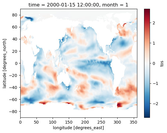
month (time) int64 1kB 1 2 3 4 5 6 7 8 9 10 11 ... 3 4 5 6 7 8 9 10 11 12Visualization#
# Plot the first time slice of the calculated anomalies
tos_anom.isel(time=0).plot()
<matplotlib.collections.QuadMesh at 0x7f2d93ab72f0>
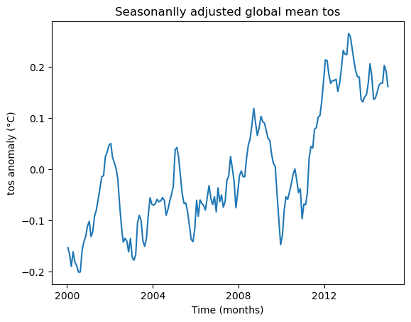
Removing Annual Cycle#
Also known as seasonal adjustment or deseasonalization, it is often used to examine underlying trends in data with a repeating cycle.
from pythia_datasets import DATASETS
import xarray as xr

# Get data
filepath = DATASETS.fetch("CESM2_sst_data.nc")
ds = xr.open_dataset(filepath)

# Remove annual cycle from the global monthly mean tos
tos_monthly = ds.tos.groupby(ds.time.dt.month)
tos_clim = tos_monthly.mean(dim="time")
tos_anom = tos_monthly - tos_clim
tos_rmAnnCyc = tos_anom.mean(dim=["lat", "lon"])

tos_rmAnnCyc
/home/runner/micromamba/envs/geocat-applications/lib/python3.12/site-packages/xarray/conventions.py:286: SerializationWarning: variable 'tos' has multiple fill values {1e+20, 1e+20} defined, decoding all values to NaN.
  var = coder.decode(var, name=name)
<xarray.DataArray 'tos' (time: 180)> Size: 720B
array([-0.15282594, -0.16537704, -0.18962625, -0.16086924, -0.18127483,
       -0.18800849, -0.2007687 , -0.20025028, -0.15869197, -0.14112295,
       -0.13107252, -0.11059521, -0.10135283, -0.1312863 , -0.12155499,
       -0.0912946 , -0.07899683, -0.05883313, -0.03680199, -0.01390849,
       -0.01227668,  0.02499827,  0.03395049,  0.04679755,  0.05092119,
        0.02437359,  0.01368596,  0.00239054, -0.01854431, -0.06873415,
       -0.1104847 , -0.14208376, -0.13456087, -0.13998358, -0.16103725,
       -0.13475642, -0.17224154, -0.17727599, -0.16723025, -0.1052778 ,
       -0.08968095, -0.09918819, -0.13901192, -0.1504459 , -0.13417733,
       -0.08904682, -0.05509104, -0.06808048, -0.07002565, -0.06656591,
       -0.05815693, -0.06311394, -0.06135486, -0.05490279, -0.06033276,
       -0.08949601, -0.07795419, -0.06166805, -0.04883578, -0.03290384,
        0.0380763 ,  0.0431514 ,  0.02393223, -0.01118076, -0.04739161,
       -0.06607009, -0.06536946, -0.08318751, -0.10946001, -0.13690935,
       -0.14107347, -0.11620697, -0.06021871, -0.09142467, -0.05940771,
       -0.06655996, -0.07023349, -0.07934014, -0.05463445, -0.03133066,
       -0.05679512, -0.0686381 , -0.05323718, -0.08291537, -0.03600609,
       -0.06290644, -0.04969135, -0.073707  , -0.0632659 , -0.02080832,
       -0.01307175,  0.02537888,  0.00276066, -0.02371201, -0.07489486,
       -0.04573968, -0.01168114, -0.00279297, -0.01410041, -0.01418451,
        0.02279471,  0.04812112,  0.05982114,  0.08840058,  0.1194719 ,
        0.09039218,  0.0663529 ,  0.08146002,  0.1038119 ,  0.0931318 ,
        0.09087274,  0.07599637,  0.0606502 ,  0.0569843 ,  0.02904456,
        0.01179023,  0.00578382, -0.04762448, -0.0981068 , -0.14708425,
       -0.12853949, -0.08007333, -0.05338066, -0.05839834, -0.04359579,
       -0.02803821, -0.00951875,  0.00107727, -0.01986883, -0.04520324,
       -0.03765109, -0.09604639, -0.06781675, -0.0687421 , -0.04520762,
        0.02323599,  0.04496676,  0.04195602,  0.07860961,  0.0818129 ,
        0.10208507,  0.10553184,  0.13360539,  0.17255165,  0.21431395,
        0.21307217,  0.18629369,  0.16850702,  0.17341022,  0.17381915,
        0.17663184,  0.15263584,  0.16835593,  0.19754802,  0.23282564,
        0.22533982,  0.22437382,  0.2661041 ,  0.26009095,  0.23738673,
        0.21331541,  0.19242647,  0.18151194,  0.18060416,  0.13666095,
        0.13193358,  0.14193751,  0.14605132,  0.16921088,  0.20661172,
        0.1834804 ,  0.13706945,  0.1392012 ,  0.15061659,  0.16437544,
        0.16900271,  0.1686668 ,  0.20350453,  0.19232802,  0.16212833],
      dtype=float32)
Coordinates:
  * time     (time) object 1kB 2000-01-15 12:00:00 ... 2014-12-15 12:00:00
month (time) int64 1kB 1 2 3 4 5 6 7 8 9 10 11 ... 3 4 5 6 7 8 9 10 11 12Visualization#
# Plot the global mean tos with the annual cycle removed
tos_rmAnnCyc.plot()
plt.title("Seasonanlly adjusted global mean tos")
plt.ylabel("tos anomaly (°C)")
plt.xlabel("Time (months)")
Text(0.5, 0, 'Time (months)')
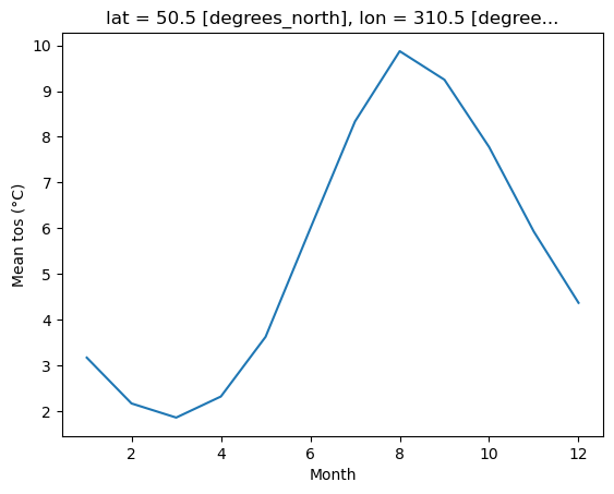
Calculating Long Term Means#
from pythia_datasets import DATASETS
import xarray as xr
import matplotlib.pyplot as plt

# Get data
filepath = DATASETS.fetch("CESM2_sst_data.nc")
ds = xr.open_dataset(filepath)

# Calculate long term mean
tos_monthly = ds.tos.groupby(ds.time.dt.month)
tos_clim = tos_monthly.mean(dim="time")

tos_clim
/home/runner/micromamba/envs/geocat-applications/lib/python3.12/site-packages/xarray/conventions.py:286: SerializationWarning: variable 'tos' has multiple fill values {1e+20, 1e+20} defined, decoding all values to NaN.
  var = coder.decode(var, name=name)
<xarray.DataArray 'tos' (month: 12, lat: 180, lon: 360)> Size: 3MB
array([[[       nan,        nan,        nan, ...,        nan,
                nan,        nan],
        [       nan,        nan,        nan, ...,        nan,
                nan,        nan],
        [       nan,        nan,        nan, ...,        nan,
                nan,        nan],
        ...,
        [-1.780786 , -1.780688 , -1.7805718, ..., -1.7809757,
         -1.7809197, -1.7808627],
        [-1.7745041, -1.7744204, -1.7743237, ..., -1.77467  ,
         -1.774626 , -1.7745715],
        [-1.7691481, -1.7690798, -1.7690051, ..., -1.7693441,
         -1.7692844, -1.7692182]],

       [[       nan,        nan,        nan, ...,        nan,
                nan,        nan],
        [       nan,        nan,        nan, ...,        nan,
                nan,        nan],
        [       nan,        nan,        nan, ...,        nan,
                nan,        nan],
...
        [-1.7605033, -1.760397 , -1.7602725, ..., -1.760718 ,
         -1.7606541, -1.7605885],
        [-1.7544289, -1.7543424, -1.7542422, ..., -1.754608 ,
         -1.754559 , -1.7545002],
        [-1.7492163, -1.749148 , -1.7490736, ..., -1.7494118,
         -1.7493519, -1.7492864]],

       [[       nan,        nan,        nan, ...,        nan,
                nan,        nan],
        [       nan,        nan,        nan, ...,        nan,
                nan,        nan],
        [       nan,        nan,        nan, ...,        nan,
                nan,        nan],
        ...,
        [-1.7711828, -1.7710832, -1.7709653, ..., -1.7713748,
         -1.7713183, -1.7712607],
        [-1.7648666, -1.7647841, -1.7646879, ..., -1.7650299,
         -1.7649865, -1.7649331],
        [-1.759478 , -1.7594113, -1.7593384, ..., -1.7596704,
         -1.7596117, -1.759547 ]]], dtype=float32)
Coordinates:
  * lat      (lat) float64 1kB -89.5 -88.5 -87.5 -86.5 ... 86.5 87.5 88.5 89.5
  * lon      (lon) float64 3kB 0.5 1.5 2.5 3.5 4.5 ... 356.5 357.5 358.5 359.5
  * month    (month) int64 96B 1 2 3 4 5 6 7 8 9 10 11 12
Attributes: (12/19)
    cell_measures:  area: areacello
    cell_methods:   area: mean where sea time: mean
    comment:        Model data on the 1x1 grid includes values in all cells f...
    description:    This may differ from "surface temperature" in regions of ...
    frequency:      mon
    id:             tos
    ...             ...
    time_label:     time-mean
    time_title:     Temporal mean
    title:          Sea Surface Temperature
    type:           real
    units:          degC
variable_id: tosVisualization#
# Plot an example location of the calculated long term means
tos_clim.sel(lon=310, lat=50, method="nearest").plot()
plt.ylabel("Mean tos (°C)")
plt.xlabel("Month")
Text(0.5, 0, 'Month')
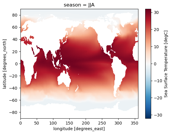
Calculating Seasonal Means#
From the xarray user guide:
The set of valid seasons consists of
‘DJF’,‘MAM’,‘JJA’and‘SON’, labeled by the first letters of the corresponding months.
If you need to work with custom seasons, the GeoCAT-comp package offers geocat.comp.climatologies.month_to_season() which can be used to create custom three-month seasonal means.
from pythia_datasets import DATASETS
import xarray as xr
import matplotlib.pyplot as plt

# Get data
filepath = DATASETS.fetch("CESM2_sst_data.nc")
ds = xr.open_dataset(filepath)

# Calculate seasonal means
tos_seasonal = ds.tos.groupby(ds.time.dt.season).mean(dim="time")

tos_seasonal
/home/runner/micromamba/envs/geocat-applications/lib/python3.12/site-packages/xarray/conventions.py:286: SerializationWarning: variable 'tos' has multiple fill values {1e+20, 1e+20} defined, decoding all values to NaN.
  var = coder.decode(var, name=name)
<xarray.DataArray 'tos' (season: 4, lat: 180, lon: 360)> Size: 1MB
array([[[       nan,        nan,        nan, ...,        nan,
                nan,        nan],
        [       nan,        nan,        nan, ...,        nan,
                nan,        nan],
        [       nan,        nan,        nan, ...,        nan,
                nan,        nan],
        ...,
        [-1.7796112, -1.779518 , -1.779407 , ..., -1.779786 ,
         -1.7797345, -1.7796829],
        [-1.7732689, -1.7731897, -1.7730962, ..., -1.7734209,
         -1.773382 , -1.7733315],
        [-1.767837 , -1.7677721, -1.7677007, ..., -1.768027 ,
         -1.7679691, -1.7679054]],

       [[       nan,        nan,        nan, ...,        nan,
                nan,        nan],
        [       nan,        nan,        nan, ...,        nan,
                nan,        nan],
        [       nan,        nan,        nan, ...,        nan,
                nan,        nan],
...
        [-1.7902642, -1.7901927, -1.7901045, ..., -1.7903785,
         -1.7903464, -1.7903149],
        [-1.7841699, -1.7841039, -1.7840254, ..., -1.7842804,
         -1.7842548, -1.7842187],
        [-1.7788147, -1.7787569, -1.7786926, ..., -1.7789872,
         -1.7789346, -1.7788768]],

       [[       nan,        nan,        nan, ...,        nan,
                nan,        nan],
        [       nan,        nan,        nan, ...,        nan,
                nan,        nan],
        [       nan,        nan,        nan, ...,        nan,
                nan,        nan],
        ...,
        [-1.6898172, -1.6897992, -1.6897855, ..., -1.6898978,
         -1.6898724, -1.6898403],
        [-1.6898259, -1.6898205, -1.6898148, ..., -1.6898614,
         -1.6898499, -1.6898375],
        [-1.6884303, -1.6883883, -1.6883432, ..., -1.6885389,
         -1.688504 , -1.6884686]]], dtype=float32)
Coordinates:
  * lat      (lat) float64 1kB -89.5 -88.5 -87.5 -86.5 ... 86.5 87.5 88.5 89.5
  * lon      (lon) float64 3kB 0.5 1.5 2.5 3.5 4.5 ... 356.5 357.5 358.5 359.5
  * season   (season) object 32B 'DJF' 'JJA' 'MAM' 'SON'
Attributes: (12/19)
    cell_measures:  area: areacello
    cell_methods:   area: mean where sea time: mean
    comment:        Model data on the 1x1 grid includes values in all cells f...
    description:    This may differ from "surface temperature" in regions of ...
    frequency:      mon
    id:             tos
    ...             ...
    time_label:     time-mean
    time_title:     Temporal mean
    title:          Sea Surface Temperature
    type:           real
    units:          degC
variable_id: tosVisualization#
# Plot the JJA time slice of the calculated seasonal means
tos_seasonal.sel(season="JJA").plot()
<matplotlib.collections.QuadMesh at 0x7f2d90e08650>
Finding The Standard Deviations of Monthly Means#
Calculate the standard deviations of monthly means for each month using the .std() function.
from pythia_datasets import DATASETS
import xarray as xr
import matplotlib.pyplot as plt

# Get data
filepath = DATASETS.fetch("CESM2_sst_data.nc")
ds = xr.open_dataset(filepath)

# Calculate the standard deviation from monthly mean data
stdMon = ds.tos.groupby(ds.time.dt.month).std()

stdMon
/home/runner/micromamba/envs/geocat-applications/lib/python3.12/site-packages/xarray/conventions.py:286: SerializationWarning: variable 'tos' has multiple fill values {1e+20, 1e+20} defined, decoding all values to NaN.
  var = coder.decode(var, name=name)
<xarray.DataArray 'tos' (month: 12, lat: 180, lon: 360)> Size: 3MB
array([[[       nan,        nan,        nan, ...,        nan,
                nan,        nan],
        [       nan,        nan,        nan, ...,        nan,
                nan,        nan],
        [       nan,        nan,        nan, ...,        nan,
                nan,        nan],
        ...,
        [0.0111143 , 0.01110211, 0.01108894, ..., 0.01114661,
         0.01113714, 0.01112626],
        [0.01120422, 0.01120154, 0.01119892, ..., 0.01121121,
         0.01120882, 0.01120653],
        [0.01111255, 0.01111323, 0.0111138 , ..., 0.01111099,
         0.01111163, 0.01111213]],

       [[       nan,        nan,        nan, ...,        nan,
                nan,        nan],
        [       nan,        nan,        nan, ...,        nan,
                nan,        nan],
        [       nan,        nan,        nan, ...,        nan,
                nan,        nan],
...
        [0.01198388, 0.01194896, 0.01191089, ..., 0.01207829,
         0.01204922, 0.01201763],
        [0.01188368, 0.01186803, 0.01185198, ..., 0.0119278 ,
         0.01191334, 0.01189866],
        [0.01157325, 0.01156648, 0.01155913, ..., 0.01159005,
         0.01158492, 0.01157935]],

       [[       nan,        nan,        nan, ...,        nan,
                nan,        nan],
        [       nan,        nan,        nan, ...,        nan,
                nan,        nan],
        [       nan,        nan,        nan, ...,        nan,
                nan,        nan],
        ...,
        [0.01126678, 0.01123608, 0.0112022 , ..., 0.01135061,
         0.01132471, 0.01129662],
        [0.01123642, 0.01122155, 0.01120648, ..., 0.01127947,
         0.0112652 , 0.01125085],
        [0.01104772, 0.0110411 , 0.01103405, ..., 0.01106357,
         0.01105863, 0.01105339]]], dtype=float32)
Coordinates:
  * lat      (lat) float64 1kB -89.5 -88.5 -87.5 -86.5 ... 86.5 87.5 88.5 89.5
  * lon      (lon) float64 3kB 0.5 1.5 2.5 3.5 4.5 ... 356.5 357.5 358.5 359.5
  * month    (month) int64 96B 1 2 3 4 5 6 7 8 9 10 11 12
Attributes: (12/19)
    cell_measures:  area: areacello
    cell_methods:   area: mean where sea time: mean
    comment:        Model data on the 1x1 grid includes values in all cells f...
    description:    This may differ from "surface temperature" in regions of ...
    frequency:      mon
    id:             tos
    ...             ...
    time_label:     time-mean
    time_title:     Temporal mean
    title:          Sea Surface Temperature
    type:           real
    units:          degC
variable_id: tosVisualization#
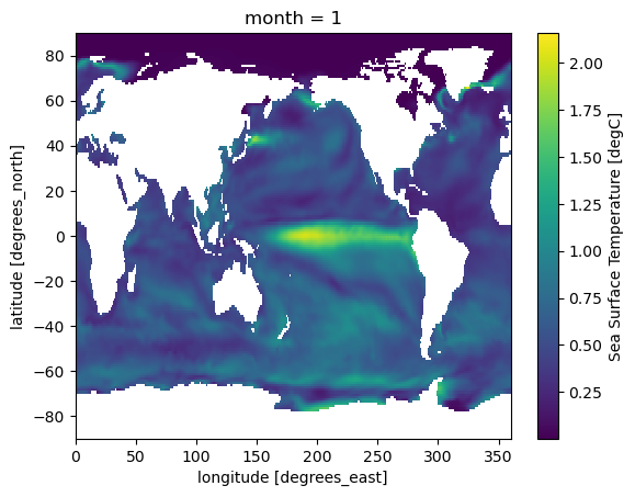
# Plot the January time slice of the calculated standard deviaitons
stdMon.sel(month=1).plot()
<matplotlib.collections.QuadMesh at 0x7f2d90d24590>
Curated Resources#
To learn more about calculating climatologies in Python, we suggest:
This Climatematch Academy notebook on xarray Data Analysis and Climatology
This Project Pythia Foundations tutorial on Computations and Masks with xarray
The xarray user guide on working with time series data