
wavelet#
Overview#
Computes the wavelet of time-series data
NCL wavelet
PyWavelets: Morlet Wavelet#
The Morlet wavelet is a complex wavelet, with both a real and imaginary component. In PyWavelets this is known as a Complex Morlet ("cmor").
NCL Morlet wavelet is based on “A Practical Guide to Wavelet Analysis” (Torrence and Compo). However, PyWavelets functions are derived from “Computational Signal Processing with Wavelets” (Teolis) to be compatible with how Matlab is defined.
To match the expected behavior of PyWavelets best to Torrence and Compo, the differences will be noted below.
Define the Complex Morlet#
PyWavelets defines a Complex Morlet Mother wavelet as cmorB-C where B is the bandwidth and C is the center frequency.
To match the Morlet wavelet function being used by NCL (Torrence and Compo, Table 1) and the PyWavelets complex morlet (Teolis, pg. 65-66), set bandwidth value B=sqrt(pi) and center frequency C=6/2*pi
# Compare Complex Morlet NCL to PyWavelets
import pywt  # PyWavelets
import numpy as np
import math
import cmath
import matplotlib.pyplot as plt  # plot data


def complex_morlet_pywavelets(time_step, B, C):
    # https://pywavelets.readthedocs.io/en/latest/ref/cwt.html#complex-morlet-wavelets
    part1 = 1 / np.sqrt(math.pi * B)
    part2 = math.exp(-np.power(time_step, 2) / B)
    part3 = cmath.exp(1j * 2 * math.pi * C * time_step)
    return part1 * part2 * part3


def tc_morlet(time_step):
    # Table 1: https://psl.noaa.gov/people/gilbert.p.compo/Torrence_compo1998.pdf
    i = np.sqrt(-1 + 0j)  # complex i
    omega = 6  # w, nondimensional frequency, defaults to 6 (~2pi)
    eta = time_step  # n, wavelet function nondimensional "time" parameter
    part1 = np.power(math.pi, -1 / 4)
    part2 = cmath.exp(i * omega * eta)
    part3 = math.exp(-np.power(eta, 2) / 2)
    return part1 * part2 * part3


def morlet_pywavelets(time_step):
    # https://pywavelets.readthedocs.io/en/latest/ref/cwt.html#morlet-wavelet
    # 'morl'
    part1 = math.exp(-np.power(time_step, 2) / 2)
    part2 = math.cos(5 * time_step)
    return part1 * part2


bandwidth = 2
center_freq = 6 / (2 * math.pi)  # C * 2 * pi = 2 * pi = approx 6 (morlet default)
amp_multiply = math.sqrt(2) * np.power(math.pi, 1 / 4)

complex_morlet = f"cmor{bandwidth}-{center_freq}"
[psi, x] = pywt.ContinuousWavelet(complex_morlet).wavefun(10)
[psi_default, x_default] = pywt.ContinuousWavelet(
    f"cmor{math.sqrt(math.pi)}-{center_freq}"
).wavefun(10)
[psi_m, x_m] = pywt.ContinuousWavelet('morl').wavefun(10)

tc_output = []
mor_pywt_output = []
cmor_pywt_output = []
for x_value in x:
    tc_output.append(tc_morlet(x_value))
    mor_pywt_output.append(morlet_pywavelets(x_value))
    cmor_pywt_output.append(complex_morlet_pywavelets(x_value, bandwidth, center_freq))

fig, ax = plt.subplots(figsize=(10, 10))
ax.plot(x, np.real(psi_default), label="PYWT cmorSQRT(pi)-6/(2*pi)", c="green")
ax.plot(x, np.real(tc_output), label="TC Morlet", c="red")
plt.title(f"PYWT cmor{math.sqrt(math.pi)}-{6/(2*math.pi)} and TC (Complex) Morlet")
ax.axhline(0, linestyle='--', alpha=0.3)
ax.legend()
plt.show()
---------------------------------------------------------------------------
ModuleNotFoundError                       Traceback (most recent call last)
Cell In[1], line 2
      1 # Compare Complex Morlet NCL to PyWavelets
----> 2 import pywt  # PyWavelets
      3 import numpy as np
      4 import math

ModuleNotFoundError: No module named 'pywt'
Note#
The Complex Morlet in PyWavelets will match along the x-intercept, but will be a smaller amplitude by 2 * fourth root of pi. The x-intercepts are the most important feature of the wavelet, but to match completely set bandwidth B=2 and multiple entire output by math.sqrt(2)*np.power(math.pi, 1/4)
Grab and Go#
import math # access to pi and square root (math.pi, math.sqrt)
import numpy as np # access to complex numbers (real and imaginary)
import cmaps # access to NCL default plot colors
import matplotlib.pyplot as plt # plot data
import geocat.datafiles as gcd # accessing nino 3 data file
import pywt # PyWavelets
# Download nino3 data
nino3_data = gcd.get('ascii_files/sst_nino3.dat')
sst_data = np.loadtxt(nino3_data)
bandwidth = math.sqrt(math.pi)
center_freq = 6 / (2 * math.pi)
wavelet_mother = f"cmor{bandwidth}-{center_freq}"
# PyWavelet Input Values
dt = 0.25 # sampling period (time between each y-value)
s0 = 0.25 # smallest scale
dj = 0.25 # spacing between each discrete scales
jtot = 44 # largest scale
scales = np.arange(1, jtot + 1, dj)
# PyWavelets
wavelet_coeffs, freqs = pywt.cwt(
data=sst_data, scales=scales, wavelet=wavelet_mother, sampling_period=dt
)
# compare the power spectrum (absolute value squared)
power = np.power((abs(wavelet_coeffs)), 2)
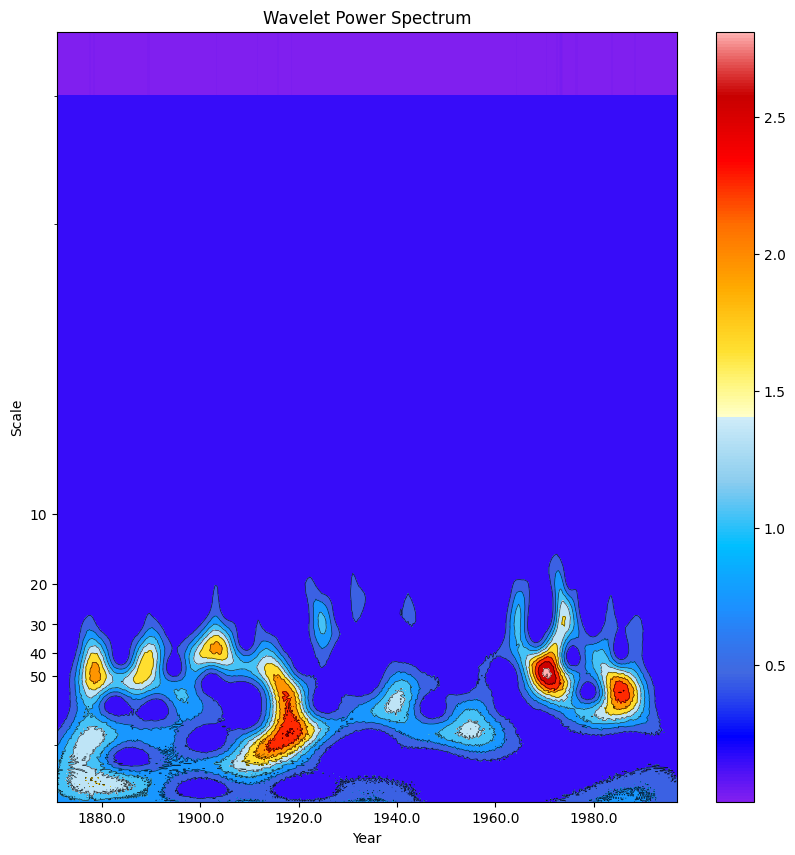
# Plot Power spectrum
fig, ax = plt.subplots(figsize=(10, 10))
# Convert Y-Axis from default to symmetrical log (symlog) with labels
ax.set_yscale("symlog")
ax.invert_yaxis()
ax.set_yticks([10, 20, 30, 40, 50])
ax.set_yticklabels([10, 20, 30, 40, 50])
# Plot contour around data
plt.contourf(
power, vmax=(power).max(), vmin=(power).min(), cmap=cmaps.ncl_default, levels=10
)
plt.contour(power, levels=10, colors="k", linewidths=0.5, alpha=0.75)
# Plot Scalogram
plt.imshow(
power, vmax=(power).max(), vmin=(power).min(), cmap=cmaps.ncl_default, aspect="auto"
)
# Convert default X-axis from time steps of 0-504 (0-len(sst_data)) to Years
start_year = 1871
end_year = 1871 + (len(sst_data) * dt)
x_tickrange = np.arange(start_year, end_year, dt)
start = int(9 / dt) # 36, starts the x-axis label at 1880 (9 years after start of data)
display_nth = int(20 / dt) # 80, display x-axis label every 20 years
plt.xticks(range(len(x_tickrange))[start::display_nth], x_tickrange[start::display_nth])
plt.title("Wavelet Power Spectrum")
plt.xlabel("Year")
plt.ylabel("Scale")
plt.colorbar()
plt.show()
Python changes to approximate NCL functionality#
# Set up `cmor` Complex Morlet to match x-intercept of NCL
bandwidth = math.sqrt(math.pi)
center_freq = 6 / (2 * math.pi)
wavelet_mother = f"cmor{bandwidth}-{center_freq}"
print(wavelet_mother)
cmor1.7724538509055159-0.954929658551372