Working with Curly Vectors

Overview

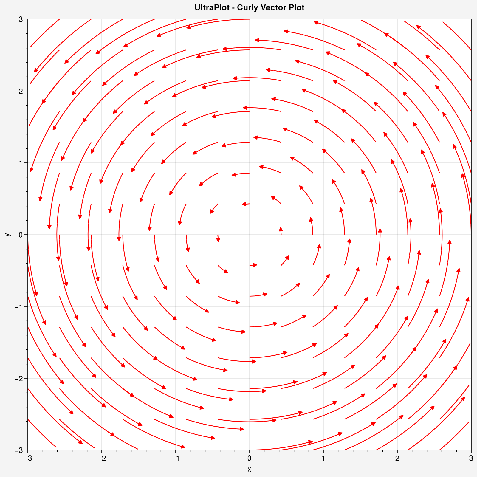
By default, plotting with packages like Matplotlib use staight lines to display vectors. Curly vectors create curved arrows that follow the vector field lines. The length of the arrow is proportional to the vector’s magnitude. This creates an intuitive way to visualize vector data commonly used in atmospheric data

Ultraplot

Ultraplot is a wrapper for Matplotlib. Curly vectors can be created via the curved_quiver()

import numpy as np
import matplotlib.pyplot as plt
import ultraplot as uplot

uplot.rc["cmap"] = "inferno"

# Sample data
x = np.linspace(-3, 3, 30)
y = np.linspace(-3, 3, 30)
X, Y = np.meshgrid(x, y)
v = X  # the y-component
u = -Y  # the x-component

# plot
fig, ax = uplot.subplot(figsize=(8, 8))

ax.curved_quiver(
    x=X,
    y=Y,
    u=u,
    v=v,
    color="red",
    arrow_at_end=True,
    arrowsize=1,
    linewidth=1,
    scale=3,
    density=3,
)

ax.format(suptitle='UltraPlot - Curly Vector Plot', grid=True, xlabel='x', ylabel='y')

plt.show()

/home/runner/micromamba/envs/geocat-applications/lib/python3.14/site-packages/ultraplot/__init__.py:223: UltraPlotWarning: Rebuilding font cache. This usually happens after installing or updating ultraplot.
  register_fonts(default=True)

Ultraplot arguments:

• x, y = Grid coordinates

• u, v = Vector components

• color = color of the arrows

• density = controls how dense the arrows are displayed as

• grains = number of seed points in x and y

• linewidth = width of arrows

• cmap, norm = colormap and normalization for array colors

• colorbar = add colorbar

• arrowsize = arrow size

• arrowstyle = arrow style

• transform = Matplotlib transform

Working with Cartopy

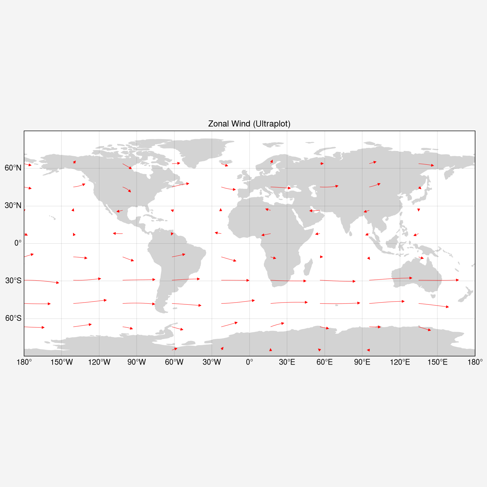
ultraplot can also overlay curly vector plots on top of world maps

Plot Vectors Globally

import geocat.datafiles as gdf  # NetCDF data files
import xarray as xr  # multi-dimensional arrays from data files

import matplotlib.pyplot as plt  # plotting
import cartopy  # plotting world maps
import ultraplot as uplot  # plotting curly vectors

# Open a netCDF data file using xarray default engine and load the data into xarrays
file_in = xr.open_dataset(gdf.get("netcdf_files/uv300.nc"))
ds = file_in.isel(time=1, lon=slice(0, -1, 3), lat=slice(1, -1, 3))

# plot
fig, ax = uplot.subplot(figsize=(8, 8), proj="cyl")

ax.add_feature(
    cartopy.feature.LAND, edgecolor='lightgray', facecolor='lightgray', zorder=0
)

ax.curved_quiver(
    ds['lon'].values,
    ds['lat'].values,
    ds['U'].values,
    ds['V'].values,
    color="red",
    arrow_at_end=True,
    arrowsize=0.7,
    linewidth=0.4,
    density=10,
    grains=10,
)

ax.format(
    land=False,
    lonlabels='bottom',  # place labels on the bottom (longitude)
    latlabels='left',  # place labels on the left (latitude)
    lonlocator=30,  # Labels every 30 degrees (longitude)
    latlocator=30,  # Labels every 30 degrees (latitude)
    lonformatter='deglon',  # Format to degrees East/West
    latformatter='deglat',  # Format to degrees North/South
)

plt.title("Zonal Wind (Ultraplot)")
plt.show()

Downloading file 'registry.txt' from 'https://github.com/NCAR/geocat-datafiles/raw/main/registry.txt' to '/home/runner/.cache/geocat'.

Downloading file 'netcdf_files/uv300.nc' from 'https://github.com/NCAR/geocat-datafiles/raw/main/netcdf_files/uv300.nc' to '/home/runner/.cache/geocat'.

/home/runner/micromamba/envs/geocat-applications/lib/python3.14/site-packages/cartopy/io/__init__.py:263: DownloadWarning: Downloading: https://naturalearth.s3.amazonaws.com/110m_physical/ne_110m_land.zip
  warnings.warn(f'Downloading: {url}', DownloadWarning)

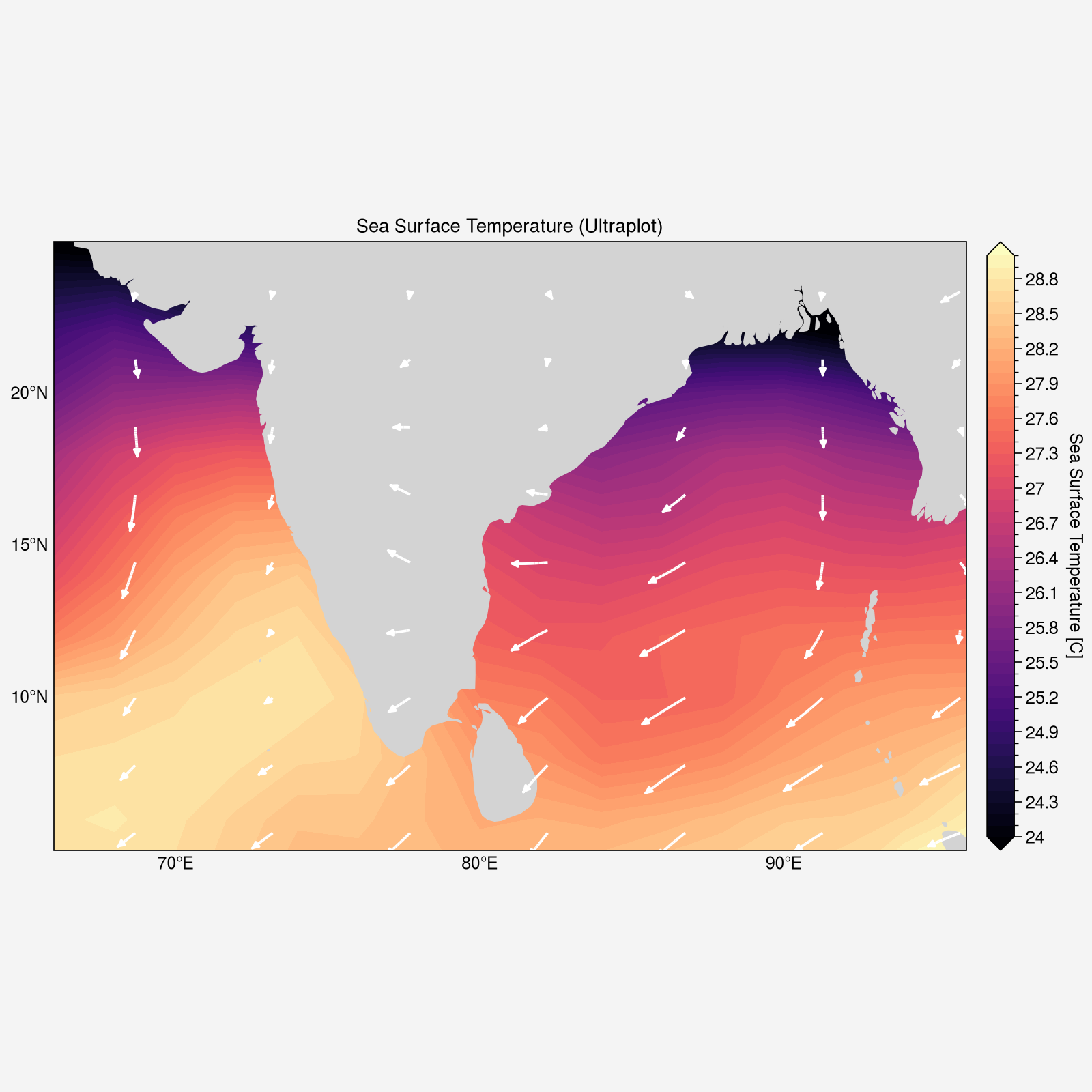
Plot Vectors on Sub-Set of Globe

import geocat.datafiles as gdf  # NetCDF data files
import xarray as xr  # multi-dimensional arrays from data files

import matplotlib.pyplot as plt  # plotting
import cartopy  # plotting world maps
import ultraplot as uplot  # plotting curly vectors

# Open a netCDF data file using xarray default engine and load the data into xarrays
sst_in = xr.open_dataset(gdf.get("netcdf_files/sst8292.nc"))
uv_in = xr.open_dataset(gdf.get("netcdf_files/uvt.nc"))

# Use date as the dimension rather than time
sst_in = sst_in.set_coords("date").swap_dims({"time": "date"}).drop_vars('time')
uv_in = uv_in.set_coords("date").swap_dims({"time": "date"}).drop_vars('time')

# Extract required variables
# Read SST and U, V for Jan 1988 (at 1000 mb for U, V)
# Note that we could use .isel() if we know the indices of date and lev
sst = sst_in['SST'].sel(date=198801)
u = uv_in['U'].sel(date=198801, lev=1000)
v = uv_in['V'].sel(date=198801, lev=1000)

# Read in grid information
lat_uv = u['lat']
lon_uv = u['lon']

# plot
fig, ax = uplot.subplot(figsize=(8, 8), proj="cyl")
ax.set_extent((66, 96, 5, 25))  # zoom on India

# Create the filled contour plot with "magma"
sst_plot = sst.plot.contourf(
    ax=ax,
    transform="cyl",
    levels=51,
    vmin=24,
    vmax=29,
    cmap="magma",
)

ax.add_feature(
    cartopy.feature.LAND, edgecolor='lightgray', facecolor='lightgray', zorder=1
)

ax.curved_quiver(
    lon_uv.values,
    lat_uv.values,
    u.values,
    v.values,
    color="white",
    arrow_at_end=True,
    arrowsize=0.7,
    linewidth=1.4,
    density=80,
    grains=80,
)

ax.format(
    title="Sea Surface Temperature (Ultraplot)",
    land=False,
    grid=False,
    lonlabels='bottom',  # place labels on the bottom (longitude)
    latlabels='left',  # place labels on the left (latitude)
    lonlocator=10,  # Labels every 10 degrees (longitude)
    latlocator=5,  # Labels every 5 degrees (latitude)
    lonformatter='deglon',  # Format to degrees East/West
    latformatter='deglat',  # Format to degrees North/South
)

plt.show()

Downloading file 'netcdf_files/sst8292.nc' from 'https://github.com/NCAR/geocat-datafiles/raw/main/netcdf_files/sst8292.nc' to '/home/runner/.cache/geocat'.

Downloading file 'netcdf_files/uvt.nc' from 'https://github.com/NCAR/geocat-datafiles/raw/main/netcdf_files/uvt.nc' to '/home/runner/.cache/geocat'.

/home/runner/micromamba/envs/geocat-applications/lib/python3.14/site-packages/cartopy/io/__init__.py:263: DownloadWarning: Downloading: https://naturalearth.s3.amazonaws.com/50m_physical/ne_50m_land.zip
  warnings.warn(f'Downloading: {url}', DownloadWarning)

Curated Resources

• NCL-inspired curly vectors: Skyborn

• GeoCAT-examples: Vector Plots