Meteorology

Overview

This section covers meteorology functions from NCL:

• dewtemp_trh

• daylight_fao56

• satvpr_temp_fao56

• satvpr_tdew_fao56

• satvpr_slope_fao56

• coriolis_param

• relhum

• relhum_ice

• relhum_water

• dpres_plevel

• psychro_fao56

dewtemp_trh

NCL’s dewtemp_trh calculates the dew point temperature given temperature and relative humidity using the equations from John Dutton’s “Ceaseless Wind” (pg. 273-274)[1] and returns a temperature in Kelvin.

Where, for the gas constant of water vapor (\(R_{v}\))of 461.5 \(\frac{J}{K*kg}\) (\(\frac{461.5}{1000 * 4.186} \frac{cal}{g*k}\)), the empirical value of the latent heat (pg. 273, Problem 8.3.1) is:

\(L_{lv} = 597.3 - 0.57(T - 273)\)

So, when \(h\) is the relative humidity, the dew point temperature (pg. 273, Equation 6, solved for as \(T_D\)) is:

\(T_D = \frac{T * L_{lv}}{L_{lv} - R_{v}Tlog(h)}\)

Important Note

To convert from Kelvin to Celsius -273.15 and to convert from Celsius to Kelvin +273.15

Grab and Go

# Input: Single Value
from geocat.comp import dewtemp

temp_c = 18  # Celsius
relative_humidity = 46.5  # %

dewtemp(temp_c + 273.15, relative_humidity) - 273.15  # Returns in Celsius

np.float64(6.298141316024157)

# Input: List/Array
from geocat.comp import dewtemp

temp_kelvin = [291.15, 274.14, 360.3, 314]  # Kelvin
relative_humidity = [46.5, 5, 96.5, 1]  # %

dewtemp(temp_kelvin, relative_humidity) - 273.15  # Returns in Celsius

array([  6.29814132, -35.12955277,  86.22114845, -27.40981025])

daylight_fao56

NCL’s daylight_fao56 calculates the maximum number of daylight hours as described in the Food and Agriculture Organization (FAO) Irrigation and Drainage Paper 56 (Chapter 3, Equation 34) [2].

Where the maximum number of daylight hours, \(N\), is:

\(N = \frac{24}{{\pi}} {\omega}_{s}\)

And \({\omega}_{s}\) is the sunset hour angle in radians (Chapter 3, Equation 25) [2] which is calculated from the latitude of the observer on Earth (\(\varphi\)) and the sun’s declination (\(\delta\)):

\({\omega}_{s} = arccos[-tan({\varphi})tan({\delta})]\)

Grab and Go

# Input: Single Value
from geocat.comp import max_daylight

day_of_year = 246  # Sept. 3
latitude = -20  # 20 Degrees South

max_daylight(day_of_year, latitude)

array([[11.665592]], dtype=float32)

# Input: List/Array
from geocat.comp import max_daylight

# Spring Equinox (March 20), Summer Solstice (June 20), Autumn Equinox (Sept. 22), Winter Solstice (Dec. 21)
days_of_year = [79, 171, 265, 355]
latitudes = 40  # Boulder

max_daylight(days_of_year, latitudes)

array([[11.921149],
       [14.843202],
       [11.920901],
       [ 9.156431]], dtype=float32)

satvpr_temp_fao56

NCL’s satvpr_temp_fao56 calculates saturation vapor pressure using temperature as described in the Food and Agriculture Organization (FAO) Irrigation and Drainage Paper 56 (Chapter 3, Equation 11) [2].

Where the saturation vapor pressure, \(e^°\) (kPa), at air temperature \(T\) (°C) is calculated as:

\(e^°(T) = 0.6108 {\exp}[\frac{17.27T}{T + 237.3}]\)

Grab and Go

# Input: Single Value
from geocat.comp import saturation_vapor_pressure

temp = 50  # Fahrenheit

saturation_vapor_pressure(temp)

array(1.22796262)

# Input: List/Array
from geocat.comp import saturation_vapor_pressure

temp = [33, 50, 100, 212]  # Fahrenheit

saturation_vapor_pressure(temp)

array([  0.63594167,   1.22796262,   6.54556639, 102.21571649])

satvpr_tdew_fao56

NCL’s satvpr_tdew_fao56 calculates the actual saturation vapor pressure using dewpoint temperature as described in the Food and Agriculture Organization (FAO) Irrigation and Drainage Paper 56 (Chapter 3, Equation 14) [2].

Where the actual vapor pressure, \(e_{a}\) (kPa), is saturation vapor pressure at a specific dewpoint temperature, \(T_{dew}\) (°C), which is calculated as:

\(e_{a} = e^°(T_{dew}) = 0.6108 {\exp}[\frac{17.27 T_{dew}}{T_{dew} + 237.3}]\)

# Input: Single Value
from geocat.comp import actual_saturation_vapor_pressure

temp = 35  # Fahrenheit

actual_saturation_vapor_pressure(temp)

array(0.68898447)

# Input: List/Array
from geocat.comp import actual_saturation_vapor_pressure

temp = [35, 60, 80, 200]  # Fahrenheit

actual_saturation_vapor_pressure(temp)

array([ 0.68898447,  1.76730647,  3.49620825, 80.00607017])

satvpr_slope_fao56

NCL’s satvpr_slope_fao56 calculates the slope of the saturation vapor pressure curve as described in the Food and Agriculture Organization (FAO) Irrigation and Drainage Paper 56 (Chapter 3, Equation 13) [2].

Where the slope of saturation vapor pressure curve, \({\Delta}\) (kPa), at air temperature \(T\) (°C) is calculated as:

\({\Delta} = \frac{4098 (0.6108 {\exp}[\frac{17.27T}{T + 237.3}])}{(T + 237.3)^2}\)

# Input: Single Value
from geocat.comp import saturation_vapor_pressure_slope

temp = 60  # Fahrenheit

saturation_vapor_pressure_slope(temp)

array(0.11322096)

# Input: List/Array
from geocat.comp import saturation_vapor_pressure_slope

temp = [35, 60, 80, 200]  # Fahrenheit

saturation_vapor_pressure_slope(temp)

array([0.04941909, 0.11322096, 0.20552235, 2.99770999])

coriolis_param

NCL’s coriolis_param calculates the Coriolis parameter at a given latitude

The Coriolis parameter (also known as the Coriolis frequency or the Coriolis coefficient) is calculated as twice the rotation rate (\({\Omega}\)) of the Earth times the sine of the latitude (\({\varphi}\))[3]

\(f = 2{\Omega}sin({\varphi})\)

The rotation rate depends on the length of the rotation period of the Earth (T) which is defined as one sidereal day (23 hours and 56 minutes):

\({\Omega} = \frac{2 * {\pi}}{T} = 7.292\text{e-5} \frac{rad}{s}\)

# Input: Single Value
from metpy.calc import coriolis_parameter
from metpy.units import units

latitude = 40  # degrees

coriolis_parameter(latitude * units.degree).magnitude

np.float64(9.374562340818716e-05)

# Input: List/Array
from metpy.calc import coriolis_parameter
from metpy.units import units

latitude = [-20, 40, 65]  # degrees

coriolis_parameter(latitude * units.degree).magnitude

array([-4.98810043e-05,  9.37456234e-05,  1.32178012e-04])

relhum

NCL’s relhum calculates relative humidity given temperature, mixing ratio, and pressure. The percent of relative humidity (\({\Psi}\)) is based on the original NCL relhum code:

\({\Psi} = w (\frac{p - 0.378 * e_s}{0.622 * e_s}) * 100\)

Where \(w\) is the mass mixing ratio of water vapor and dry air, \(p\) is pressure, and \(e_s\) is the saturation vapor pressure for a given temperature.

The constant 0.622 represents the ratio of the molar mass of water vapor (\(M_w\)) in g/mol and the molar mass of dry air (\(M_d\)) in g/mol:

\(\frac{M_w}{M_d} = \frac{18.02}{28.9634} = 0.622\)

# Input: Single Value
from geocat.comp import relhum

temp = 303.15  # Kelvin
mixing_ratio = 0.018
pressure = 101325  # Pa

relhum(temp, mixing_ratio, pressure)

np.float64(68.05239617370448)

# Input: List/Array
from geocat.comp import relhum

temp = [375.15, 303.15, 315.15]  # Kelvin
mixing_ratio = [0.5, 0.018, 0.001]
pressure = [100325, 101325, 101400]  # Pa

relhum(temp, mixing_ratio, pressure)

array([43.78181802, 68.05239617,  1.92796564])

relhum_ice

NCL’s relhum_ice calculates relative humidity with respect to ice, given temperature, mixing ratio, and pressure.

First,the approximation of vapor pressure is calculated from the Magnus Form.[4]

\({P_v} = c \exp^{\frac{a * T}{b + T}}\)

Where \(c\) is vapor pressure of water at 0 degrees Celsius (Pa), and \(a\) and \(b\) are saturation vapor pressure coefficient approximations over ice, as defined by the AEDki model.[5]

\(a = 22.571\), \(b = 273.71\), \(c = 6.1128\)

Then, the specific humidity (\(q_{st}\)) is calculated with \(p\) as pressure:

\(q_{st} = \frac{0.622 * P_v}{(p * 0.1) - 0.378 * P_v}\)

The constant 0.622 represents the ratio of the molar mass of vapor (\(M_w\)) and dry air (\(M_d\)) in g/mol:

\(\frac{M_w}{M_d} = \frac{18.02}{28.9634} = 0.622\)

And the 0.378 represents a correction constant where:

\(1 - \frac{M_w}{M_d} = 1 - 0.622 = 0.378\)

The percent of relative humidity (\({\Psi}\)) is calculated with \(w\) as the mixing ratio:

\({\Psi} = 100 * \frac{w}{q_{st}}\)

# Input: Single Value
from geocat.comp import relhum_ice

temp = 268.15  # Kelvin
mixing_ratio = 0.0037
pressure = 100000  # Pa

relhum_ice(temp, mixing_ratio, pressure)

np.float64(147.88012516016957)

# Input: List/Array
from geocat.comp import relhum_ice

temp = [268.15, 258.15, 250.15]  # Kelvin
mixing_ratio = [0.0037, 0.018, 0.001]
pressure = [100000, 100325, 101325]  # Pa

relhum_ice(temp, mixing_ratio, pressure)

array([ 147.88012516, 1756.81983351,  211.26793555])

relhum_water

NCL’s relhum_water calculates relative humidity with respect to water, given temperature, mixing ratio, and pressure.

First,the approximation of vapor pressure is calculated from the Magnus Tetens form.[6]

\({P_v} = c \exp^{\frac{a (T- 273.16)}{T - b}}\)

Where \(c\) is vapor pressure of water at 0 degrees Celsius (Pa) as defined by the AEDki model[5], and \(a\) and \(b\) are saturation vapor pressure coefficient approximations, as defined by the Magnus Tetens model (Equation 6)[6]

\(a = 17.269\), \(b = 35.86\), \(c = 6.1128\)

Then, the specific humidity (\(q_{st}\)) is calculated with \(p\) as pressure:

\(q_{st} = \frac{0.622 * P_v}{(p * 0.1) - 0.378 * P_v}\)

The constant 0.622 represents the ratio of the molar mass of vapor (\(M_w\)) and dry air (\(M_d\)) in g/mol:

\(\frac{M_w}{M_d} = \frac{18.02}{28.9634} = 0.622\)

And the 0.378 represents a correction constant where:

\(1 - \frac{M_w}{M_d} = 1 - 0.622 = 0.378\)

The percent of relative humidity (\({\Psi}\)) is calculated with \(w\) as the mixing ratio:

\({\Psi} = 100 * \frac{w}{q_{st}}\)

# Input: Single Value
from geocat.comp import relhum_water

temp = 315.15  # Kelvin
mixing_ratio = 0.0037
pressure = 100000  # Pa

relhum_water(temp, mixing_ratio, pressure)

np.float64(7.025120800518423)

# Input: List/Array
from geocat.comp import relhum_ice

temp = [298.15, 315.15, 330.15]  # Kelvin
mixing_ratio = [0.0018, 0.0037, 0.001]
pressure = [100325, 100000, 101325]  # Pa

relhum_water(temp, mixing_ratio, pressure)

array([9.04879928, 7.0251208 , 0.87910297])

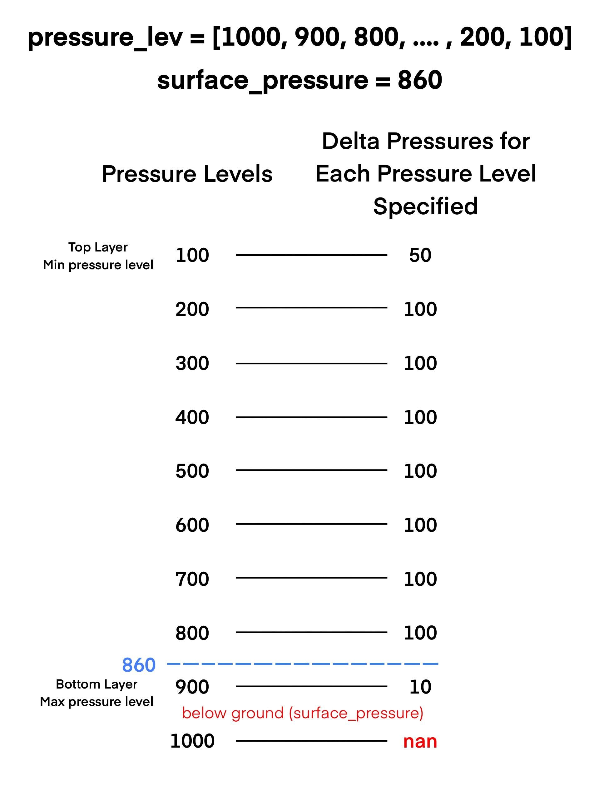
dpres_plevel

NCL’s dpres_plevel calculates the change in pressure (delta pressure) for each layer in a specified constant pressure level coordinate system while accounting for specified surface and top pressures.

Important Note

Some layers may be assigned missing values if they are fully below the ground (below surface_pressure) or fully above the specified pressure top in NCL. In geocat-comp the surface pressure is accounted for as in NCL, but the pressure top is assumed to be the minimum specified pressure level and is not currently user configurable.

For example:

# Input: Single Value
from geocat.comp import delta_pressure
import numpy as np


pressure_levels = np.array(
    [
        1000,
        950,
        900,
        850,
        800,
        750,
        700,
        650,
        600,
        550,
        500,
        450,
        400,
        350,
        300,
        250,
        200,
        175,
        150,
        125,
        100,
        80,
        70,
        60,
        50,
        40,
        30,
        25,
        20,
    ]
)
surface_pressure = 1050

delta_pressure(pressure_levels, surface_pressure)

array([75. , 50. , 50. , 50. , 50. , 50. , 50. , 50. , 50. , 50. , 50. ,
       50. , 50. , 50. , 50. , 50. , 37.5, 25. , 25. , 25. , 22.5, 15. ,
       10. , 10. , 10. , 10. ,  7.5,  5. ,  2.5])

# Input: List/Array
from geocat.comp import delta_pressure
import numpy as np

pressure_levels = np.array(
    [
        1000,
        950,
        900,
        850,
        800,
        750,
        700,
        650,
        600,
        550,
        500,
        450,
        400,
        350,
        300,
        250,
        200,
        175,
        150,
        125,
        100,
        80,
        70,
        60,
        50,
        40,
        30,
        25,
        20,
    ]
)
surface_pressure = np.array([1000, 1025, 1050])

delta_pressure(pressure_levels, surface_pressure)

array([[25. , 50. , 50. , 50. , 50. , 50. , 50. , 50. , 50. , 50. , 50. ,
        50. , 50. , 50. , 50. , 50. , 37.5, 25. , 25. , 25. , 22.5, 15. ,
        10. , 10. , 10. , 10. ,  7.5,  5. ,  2.5],
       [50. , 50. , 50. , 50. , 50. , 50. , 50. , 50. , 50. , 50. , 50. ,
        50. , 50. , 50. , 50. , 50. , 37.5, 25. , 25. , 25. , 22.5, 15. ,
        10. , 10. , 10. , 10. ,  7.5,  5. ,  2.5],
       [75. , 50. , 50. , 50. , 50. , 50. , 50. , 50. , 50. , 50. , 50. ,
        50. , 50. , 50. , 50. , 50. , 37.5, 25. , 25. , 25. , 22.5, 15. ,
        10. , 10. , 10. , 10. ,  7.5,  5. ,  2.5]])

psychro_fao56

Computes the psychrometric constant (kPa/C) as described in the Food and Agriculture Organization (FAO) Irrigation and Drainage Paper 56 (Chapter 3, Equation 8 or Equation 3-10 in Annex 3)[2].

\({\gamma} = \frac{c_{p}P}{{\epsilon}{\lambda}}\)

\({\gamma} = \frac{1.013 \text{e-3} * P}{0.622 * 2.45}\)

\({\gamma} = 0.6647 \text{e-3} * P\)

Where, \({\gamma}\) is the psychrometric constant (in kPa/C), \(P\) is the atmospheric pressure (kPa), \({\lambda}\) is the latent heat vaporization (2.45 MJ/kgC), and \({\epsilon}\) is the ratio of the molecular weight of water and dry air (0.622)

# Input: Single Value
from geocat.comp import psychrometric_constant

pressure = 80  # kPa/C
psychrometric_constant(pressure)

np.float64(0.0531792)

# Input: List/Array
from geocat.comp import psychrometric_constant

pressure = [10, 50, 80, 1000]
psychrometric_constant(pressure)

array([0.0066474, 0.033237 , 0.0531792, 0.66474  ])

---

Python Resources

• GeoCAT-comp dewtemp documentation

• Convert between different temperature scales in SciPy

• GeoCAT-comp max_daylight Documentation

• GeoCAT-comp saturation_vapor_pressure Documentation

• GeoCAT-comp actual_saturation_vapor_pressure Documentation

• GeoCAT-comp saturation_vapor_pressure_slope Documentation

• MetPy coriolis_parameter Documentation

• GeoCAT-comp relhum Documentation

• GeoCAT-comp relhum_ice Documentation

• GeoCAT-comp relhum_water Documentation

• GeoCAT-comp delta_pressure Documentation

• GeoCAT-comp psychrometric_constant Documentation

Additional Reading

• NOAA: Dew Point vs. Humidity

• MetPy relative_humidity_from_mixing_ratio Documentation with alternative equation

References:

---

[1]

John A. Dutton. The Ceaseless Wind: An Introduction to the Theory of Atmospheric Motion. Dover Publications, 1986.

[2] (1,2,3,4,5,6)

Richard Allan, L. Pereira, and Martin Smith. Crop evapotranspiration - Guidelines for computing crop water requirements - FAO Irrigation and drainage paper 56. Volume 56. FAO, 01 1998.

[3]

Peter V. Hobbs and John Michael Wallace. Atmospheric Science: An Introductory Survey. Academic Press, 1977.

[4]

Oleg A Alduchov and Robert E. Eskridge. Improved magnus form approximation of saturation vapor pressure. 1997. doi:10.2172/548871.

[5] (1,2)

Oleg A Alduchov and Robert E. Eskridge. Notes and correspondence: improved magnus form approximation of saturation vapor pressure. 1996. doi:10.1175/1520-0450(1996)035%3C0601:IMFAOS%3E2.0.CO;2.

[6] (1,2)

F. W. Murray. On the computation of saturation vapor pressure. 1967. doi:10.1175/1520-0450(1967)006%3C0203:OTCOSV%3E2.0.CO;2.