specx_anal

Warning

This is not meant to be a standalone notebook. This notebook is part of the process we have for adding entries to the NCL Index and is not meant to be used as tutorial or example code.

import xarray as xr
import geocat.datafiles as gcd
import pandas as pd
import scipy
import matplotlib.pyplot as plt
import numpy as np

NCL code

;*************************************************
; spec_1.ncl
;
; Concepts illustrated:
;   - Calculating and plotting spectra
;************************************************
;
; These files are loaded by default in NCL V6.2.0 and newer
; load "$NCARG_ROOT/lib/ncarg/nclscripts/csm/gsn_code.ncl"
; load "$NCARG_ROOT/lib/ncarg/nclscripts/csm/gsn_csm.ncl" 
;************************************************
begin
;************************************************
; variable and file handling
;************************************************
   fn  = "SOI_Darwin.nc" ; define filename
   in  = addfile(fn,"r")                                 ; open netcdf file
   soi  = in->DSOI                                       ; get data
;************************************************
; set function arguments
;************************************************
; detrending opt: 0=>remove mean 1=>remove mean and detrend
  d = 0
; smoothing periodogram: (0 <= sm <= ??.) should be at least 3 and odd
  sm = 7
; percent tapered: (0.0 <= pct <= 1.0) 0.10 common. 
  pct = 0.10
;************************************************
; calculate spectrum
;************************************************
  spec = specx_anal(soi,d,sm,pct)
;************************************************
; plotting
;************************************************
   wks  = gsn_open_wks("png","spec")               ; send graphics to PNG file 

   res = True					   ; plot mods desired
   res@tiMainString = "SOI"		           ; title
   res@tiXAxisString = "Frequency (cycles/month)"  ; xaxis
   res@tiYAxisString = "Variance"                  ; yaxis

   plot=gsn_csm_xy(wks,spec@frq,spec@spcx,res)     ; create plot   
;***********************************************
end

Python Functionality

soi_darwin = xr.open_dataset(gcd.get('netcdf_files/SOI_Darwin.nc'))

soi_darwin

<xarray.Dataset> Size: 22kB
Dimensions:  (time: 1404)
Coordinates:
  * time     (time) int32 6kB 0 1 2 3 4 5 6 ... 1398 1399 1400 1401 1402 1403
Data variables:
    date     (time) float64 11kB ...
    DSOI     (time) float32 6kB ...
Attributes:
    title:          Darwin Southern Oscillation Index
    source:         Climate Analysis Section, NCAR
    history:        \nDSOI = - Normalized Darwin\nNormalized sea level pressu...
    creation_date:  Tue Mar 30 09:29:20 MST 1999
    references:     Trenberth, Mon. Wea. Rev: 2/1984
    time_span:      1882 - 1998
    conventions:    None

xarray.Dataset

• Dimensions:
  • time: 1404
• Coordinates: (1)
  • time
    (time)
    int32
    0 1 2 3 4 ... 1400 1401 1402 1403

    long_name :

    Months Since January 1882

    units :

    months

    array([   0,    1,    2, ..., 1401, 1402, 1403], dtype=int32)

• Data variables: (2)
  • date
    (time)
    float64
    ...

    short_name :

    Yr-Mo

    long_name :

    Year-Month

    units :

    YYYYMM

    [1404 values with dtype=float64]

  • DSOI
    (time)
    float32
    ...

    short_name :

    DSOI

    long_name :

    Darwin Southern Oscillation Index

    units :

    dimensionless

    [1404 values with dtype=float32]

• Indexes: (1)
  • time
    PandasIndex

    PandasIndex(Index([   0,    1,    2,    3,    4,    5,    6,    7,    8,    9,
           ...
           1394, 1395, 1396, 1397, 1398, 1399, 1400, 1401, 1402, 1403],
          dtype='int32', name='time', length=1404))

• Attributes: (7)

  title :

  Darwin Southern Oscillation Index

  source :

  Climate Analysis Section, NCAR

  history :

  DSOI = - Normalized Darwin Normalized sea level pressure is used. The normalization is done using Trenberth's method. Briefly, the overall anomaly standard dev for Darwin is used to normalize rather than the st dev of each month's anomaly. This optimizes the signal-to-noise ratio. see http://www.cgd.ucar.edu/cas/climind/soi.html

  creation_date :

  Tue Mar 30 09:29:20 MST 1999

  references :

  Trenberth, Mon. Wea. Rev: 2/1984

  time_span :

  1882 - 1998

  conventions :

  None

start_date = pd.Timestamp('1882-01-01')
dates = [
    start_date + pd.DateOffset(months=int(month))
    for month in soi_darwin.indexes['time']
]
datetime_index = pd.DatetimeIndex(dates)

datetime_index

DatetimeIndex(['1882-01-01', '1882-02-01', '1882-03-01', '1882-04-01',
               '1882-05-01', '1882-06-01', '1882-07-01', '1882-08-01',
               '1882-09-01', '1882-10-01',
               ...
               '1998-03-01', '1998-04-01', '1998-05-01', '1998-06-01',
               '1998-07-01', '1998-08-01', '1998-09-01', '1998-10-01',
               '1998-11-01', '1998-12-01'],
              dtype='datetime64[ns]', length=1404, freq=None)

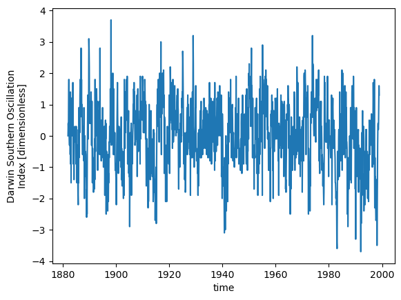
soi = soi_darwin.DSOI
soi['time'] = datetime_index

soi.plot();

soi_detrended = scipy.signal.detrend(soi, type='constant')

percent_taper = 0.1
tukey_window = scipy.signal.windows.tukey(
    len(soi_detrended), alpha=percent_taper, sym=False
)  # generates a periodic window

soi_tapered = soi_detrended * tukey_window

freq_soi, psd_soi = scipy.signal.periodogram(
    soi_tapered,
    fs=1,  # sample monthly
    detrend=False,
)

k = 7  # define smoothing constant

kernel = np.ones(7)  # Create a Daniel smoothing kernel
kernel[0] = (
    0.5  # "Modify" kernel by making the endpoints have half the weight of the interior points
)
kernel[-1] = 0.5
kernel = kernel / kernel.sum()

smoothed_psd = scipy.signal.convolve(
    psd_soi, kernel, mode='same'
)  # Sets output array as the same length as the first input

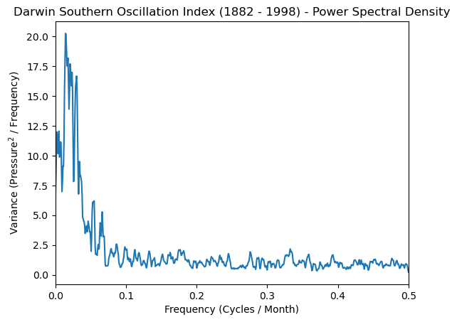
variance = np.var(soi_tapered, ddof=1)

df = freq_soi[1] - freq_soi[0]  # Frequency step

# Create an array to adjust contributions of endpoints
frac = np.ones_like(freq_soi)
frac[0] = 0.5
frac[-1] = 0.5

current_area = np.sum(
    smoothed_psd * df * frac
)  # Calculate the current area under the curve
normalization_factor = variance / current_area  # Find the factor to adjust this area

normalized_psd = (
    smoothed_psd * normalization_factor
)  # Apply the normalization factor to the smoothed power spectrum

plt.plot(freq_soi, normalized_psd)
plt.xlabel('Frequency (Cycles / Month)')
plt.ylabel('Variance (Pressure$^2$ / Frequency)')
plt.title('Darwin Southern Oscillation Index (1882 - 1998) - Power Spectral Density')
plt.xlim([0, 0.5]);

Comparison

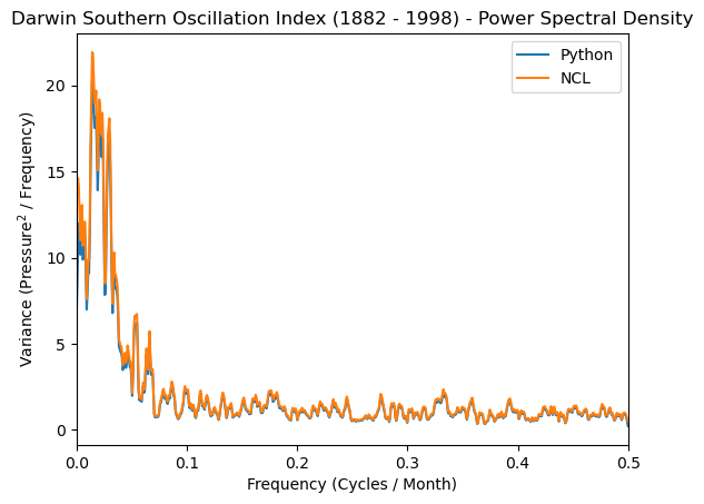
ncl = xr.open_dataset(gcd.get('applications_files/ncl_outputs/spec_1_output.nc')).spec

frq = ncl.frq
spcx = ncl.spcx

Downloading file 'applications_files/ncl_outputs/spec_1_output.nc' from 'https://github.com/NCAR/GeoCAT-datafiles/raw/main/applications_files/ncl_outputs/spec_1_output.nc' to '/home/runner/.cache/geocat'.

plt.plot(freq_soi, normalized_psd, label='Python')
plt.plot(frq, spcx, label='NCL')
plt.xlabel('Frequency (Cycles / Month)')
plt.ylabel('Variance (Pressure$^2$ / Frequency)')
plt.title('Darwin Southern Oscillation Index (1882 - 1998) - Power Spectral Density')
plt.xlim([0, 0.5])
plt.legend();

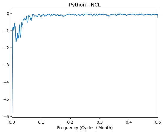
plt.plot(frq, normalized_psd[1:] - spcx)
plt.xlim([0, 0.5])
plt.title('Python - NCL')
plt.xlabel('Frequency (Cycles / Month)');

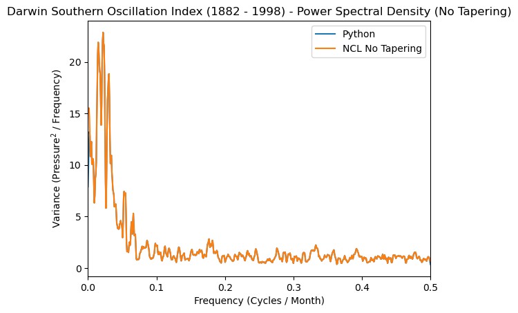
Comparison without Tapering

It is important to remember that periodograms are estimates of a spectra, and the recommended math for performing this analysis, as well as for the various window operations, has changed over the decades since NCL was written.

We have demonstrated to the best of our ability how to follow the decisions made by NCL developers and have results similar enough to be confident that this approach in Python is correct.

However, in the interest of tracking down the differences we will investigate the output from Python and NCL without tapering.

Because Tukey tapering can refer to split-bell-cosine or cosine tapering, this is the step of our workflow where NCL’s decisions are the least clear.

ncl_notaper = xr.open_dataset(
    gcd.get('applications_files/ncl_outputs/spec_1_output_notaper.nc')
).spec
spcx_nt = ncl_notaper.spcx

Downloading file 'applications_files/ncl_outputs/spec_1_output_notaper.nc' from 'https://github.com/NCAR/GeoCAT-datafiles/raw/main/applications_files/ncl_outputs/spec_1_output_notaper.nc' to '/home/runner/.cache/geocat'.

# Compute Periodogram without tapering and with mean removed
freq_soi, psd_soi_nt = scipy.signal.periodogram(
    soi_detrended,
    fs=1,  # sample monthly
    detrend=False,
)

# Smooth with the same modified Daniel kernel as before
smoothed_psd_nt = scipy.signal.convolve(psd_soi_nt, kernel, mode='same')

# Normalize
variance = np.var(soi_detrended, ddof=1)
current_area = np.sum(
    smoothed_psd_nt * df * frac
)  # Calculate the current area under the curve
normalization_factor = variance / current_area  # Find the factor to adjust this area

normalized_psd_nt = (
    smoothed_psd_nt * normalization_factor
)  # Apply the normalization factor to the smoothed power spectrum

plt.plot(freq_soi, normalized_psd_nt, label='Python')
plt.plot(frq, spcx_nt, label='NCL No Tapering')
plt.xlabel('Frequency (Cycles / Month)')
plt.ylabel('Variance (Pressure$^2$ / Frequency)')
plt.title(
    'Darwin Southern Oscillation Index (1882 - 1998) - Power Spectral Density (No Tapering)'
)
plt.xlim([0, 0.5])
plt.legend();

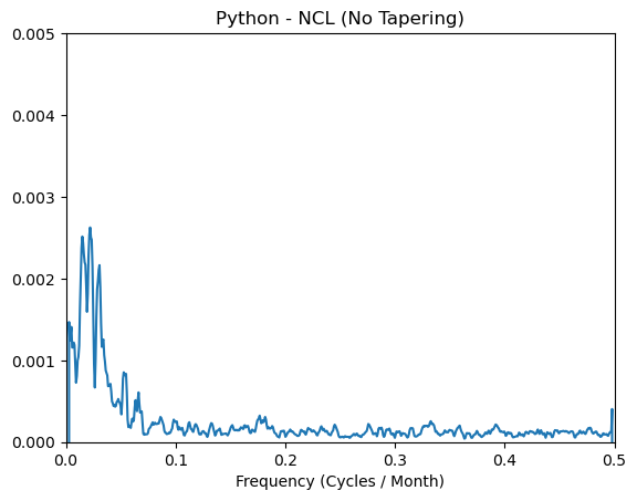
plt.plot(frq, normalized_psd_nt[1:] - spcx_nt)
plt.xlim([0, 0.5])
plt.title('Python - NCL (No Tapering)')
plt.ylim([-0.00, 0.005])
plt.xlabel('Frequency (Cycles / Month)');