Vectorized matrix solver#
Many of the tutorials have defined a chemical system without talking about their location. Each of these is essentially
defining a box model. We often want to model chemistry
in more than one location; multiple boxes. In weather and climate models, the domain is broken up into 2d or 3d grids.
Each location may be referred to as a grid cell or column. With micm, we can solve multiple grid cells simultaneously in
several ways.
The tutorials listed below solve chemistry in more than one grid cell.
Multiple Grid Cells, this tutorial does so with a different data structure
OpenMP, this tutorial uses a single thread per grid cell
In Multiple Grid Cells we assumed we were solving for the concentrations of an \(N\times D\) matrix, \(N\) species and \(D\) grid cells. However, we used the default matrix ordering in that tutorial. This is fine for simulations that aren’t too large, but computationally may be inferior. This is because the same species appears in each grid cell, \(N\) elements away from each other in memory. When solving the chemical equations, the same mathematical operations have to be applied to each species. We can organize the memory of the matrix so that the same species across all \(D\) grid cells are directly next to each other in memory. In this way, we help to encourage the compiler to vectorize the code and take advantage of SIMD instructions.
Organizing the data this way may be familiar to GPU programmers as coalesced memory access.
To understand this, we’ll look at how the memeory is organized when solving the robertson equations with 3 grid cells using
the various matrix types and ordering in micm.
This entire example is contained below. Copy and paste to follow along.
#include <micm/CPU.hpp>

#include <chrono>
#include <iomanip>
#include <iostream>

// Use our namespace so that this example is easier to read
using namespace micm;

void solve(auto& solver, auto& state, std::size_t number_of_grid_cells)
{
  double k1 = 0.04;
  double k2 = 3e7;
  double k3 = 1e4;
  state.SetCustomRateParameter("r1", std::vector<double>(3, k1));
  state.SetCustomRateParameter("r2", std::vector<double>(3, k2));
  state.SetCustomRateParameter("r3", std::vector<double>(3, k3));

  double temperature = 272.5;  // [K]
  double pressure = 101253.3;  // [Pa]
  double air_density = 1e6;    // [mol m-3]

  for (size_t cell = 0; cell < number_of_grid_cells; ++cell)
  {
    state.conditions_[cell].temperature_ = temperature;
    state.conditions_[cell].pressure_ = pressure;
    state.conditions_[cell].air_density_ = air_density;
  }

  double time_step = 100;  // s

  SolverState solver_state = SolverState::Converged;
  for (int i = 0; i < 10 && solver_state == SolverState::Converged; ++i)
  {
    double elapsed_solve_time = 0;
    solver.CalculateRateConstants(state);
    while (elapsed_solve_time < time_step && solver_state != SolverState::Converged)
    {
      auto result = solver.Solve(time_step - elapsed_solve_time, state);
      elapsed_solve_time += result.stats_.final_time_;;
      solver_state = result.state_;
    }
  }
  if (solver_state != SolverState::Converged)
  {
    throw "Solver did not converge";
  }
}

int main()
{
  auto a = Species("A");
  auto b = Species("B");
  auto c = Species("C");

  Phase gas_phase{ "gas", std::vector<PhaseSpecies>{ a, b, c } };

  Process r1 = ChemicalReactionBuilder()
                   .SetReactants({ a })
                   .SetProducts({ StoichSpecies(b, 1) })
                   .SetRateConstant(UserDefinedRateConstant({ .label_ = "r1" }))
                   .SetPhase(gas_phase)
                   .Build();

  Process r2 = ChemicalReactionBuilder()
                   .SetReactants({ b, b })
                   .SetProducts({ StoichSpecies(b, 1), StoichSpecies(c, 1) })
                   .SetRateConstant(UserDefinedRateConstant({ .label_ = "r2" }))
                   .SetPhase(gas_phase)
                   .Build();

  Process r3 = ChemicalReactionBuilder()
                   .SetReactants({ b, c })
                   .SetProducts({ StoichSpecies(a, 1), StoichSpecies(c, 1) })
                   .SetRateConstant(UserDefinedRateConstant({ .label_ = "r3" }))
                   .SetPhase(gas_phase)
                   .Build();

  auto params = RosenbrockSolverParameters::ThreeStageRosenbrockParameters();
  auto system = System(SystemParameters{ .gas_phase_ = gas_phase });
  auto reactions = std::vector<Process>{ r1, r2, r3 };
  const std::size_t number_of_grid_cells = 3;

  auto solver = CpuSolverBuilder<micm::RosenbrockSolverParameters>(params).SetSystem(system).SetReactions(reactions).Build();

  auto state = solver.GetState(number_of_grid_cells);

  state.SetConcentration(a, { 1.1, 2.1, 3.1 });
  state.SetConcentration(b, { 1.2, 2.2, 3.2 });
  state.SetConcentration(c, { 1.3, 2.3, 3.3 });

  for (auto& elem : state.variables_.AsVector())
  {
    std::cout << elem << std::endl;
  }

  std::cout << std::endl;

  auto vectorized_solver = CpuSolverBuilder<
                               RosenbrockSolverParameters,
                               VectorMatrix<double, 3>,
                               SparseMatrix<double, SparseMatrixVectorOrdering<3>>>(params)
                               .SetSystem(system)
                               .SetReactions(reactions)
                               .Build();

  auto vectorized_state = vectorized_solver.GetState(number_of_grid_cells);

  vectorized_state.SetConcentration(a, { 1.1, 2.1, 3.1 });
  vectorized_state.SetConcentration(b, { 1.2, 2.2, 3.2 });
  vectorized_state.SetConcentration(c, { 1.3, 2.3, 3.3 });

  for (auto& elem : vectorized_state.variables_.AsVector())
  {
    std::cout << elem << std::endl;
  }

  std::cout << std::endl;

  solve(solver, state, number_of_grid_cells);
  solve(vectorized_solver, vectorized_state, number_of_grid_cells);

  for (size_t cell = 0; cell < number_of_grid_cells; ++cell)
  {
    std::cout << "Cell " << cell << std::endl;
    std::cout << std::setw(10) << "Species" << std::setw(20) << "Regular" << std::setw(20) << "Vectorized" << std::endl;

    for (auto& species : system.UniqueNames())
    {
      auto regular_idx = state.variable_map_[species];
      auto vectorized_idx = vectorized_state.variable_map_[species];

      std::cout << std::setw(10) << species << std::setw(20) << state.variables_[cell][regular_idx] << std::setw(20)
                << vectorized_state.variables_[cell][vectorized_idx] << std::endl;
    }

    std::cout << std::endl;
  }

  micm::SparseMatrix<std::string> sparse_matrix{ micm::SparseMatrix<std::string>::Create(4)
                                                     .WithElement(0, 1)
                                                     .WithElement(2, 1)
                                                     .WithElement(2, 3)
                                                     .WithElement(3, 2)
                                                     .SetNumberOfBlocks(3) };

  micm::SparseMatrix<std::string, micm::SparseMatrixVectorOrdering<3>> sparse_vector_matrix{
    micm::SparseMatrix<std::string, micm::SparseMatrixVectorOrdering<3>>::Create(4)
        .WithElement(0, 1)
        .WithElement(2, 1)
        .WithElement(2, 3)
        .WithElement(3, 2)
        .SetNumberOfBlocks(3)
  };

  sparse_matrix[0][0][1] = sparse_vector_matrix[0][0][1] = "0.0.1";
  sparse_matrix[0][2][1] = sparse_vector_matrix[0][2][1] = "0.2.1";
  sparse_matrix[0][2][3] = sparse_vector_matrix[0][2][3] = "0.2.3";
  sparse_matrix[0][3][2] = sparse_vector_matrix[0][3][2] = "0.3.2";
  sparse_matrix[1][0][1] = sparse_vector_matrix[1][0][1] = "1.0.1";
  sparse_matrix[1][2][1] = sparse_vector_matrix[1][2][1] = "1.2.1";
  sparse_matrix[1][2][3] = sparse_vector_matrix[1][2][3] = "1.2.3";
  sparse_matrix[1][3][2] = sparse_vector_matrix[1][3][2] = "1.3.2";
  sparse_matrix[2][0][1] = sparse_vector_matrix[2][0][1] = "2.0.1";
  sparse_matrix[2][2][1] = sparse_vector_matrix[2][2][1] = "2.2.1";
  sparse_matrix[2][2][3] = sparse_vector_matrix[2][2][3] = "2.2.3";
  sparse_matrix[2][3][2] = sparse_vector_matrix[2][3][2] = "2.3.2";

  std::cout << std::endl << "Sparse matrix standard ordering elements" << std::endl;
  for (auto& elem : sparse_matrix.AsVector())
  {
    std::cout << elem << std::endl;
  }
  std::cout << std::endl << "Sparse matrix vector ordering elements" << std::endl;
  for (auto& elem : sparse_vector_matrix.AsVector())
  {
    std::cout << elem << std::endl;
  }
}
Matrix types in micm#
micm has its own matrix types. These provide dense matrices (for species concentrations, reaction rates, etc.),
and sparse matrices (for the Jacobian matrix).
The elements of these matrices are placed in a contiguous vector, in an effort to minimize cache misses.
Both dense and sparse matrices also have two strategies for element ordering available: standard and vector.
The vector-ordering strategy is intented to encourage vectorization of the solver code.
Dense and sparse matrix types are described in more detail below.
Dense matrix#
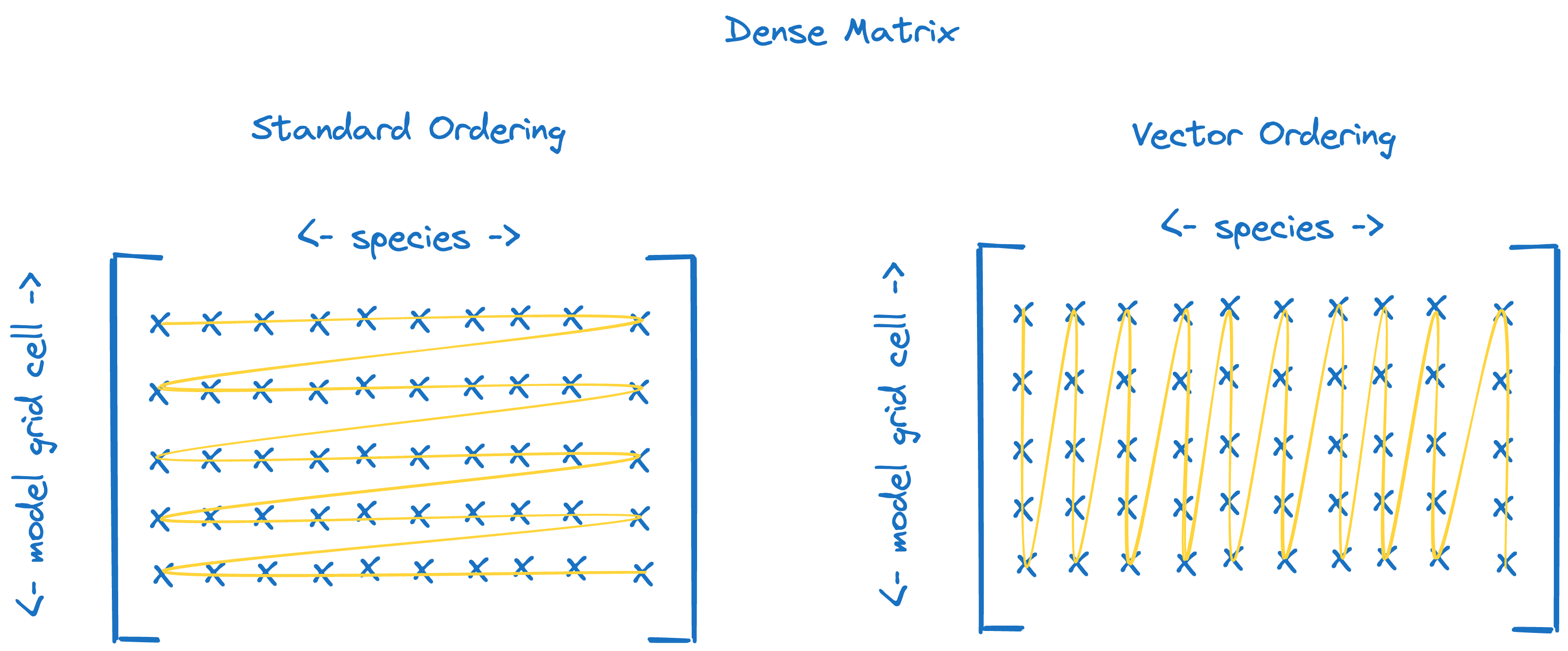
Element ordering for standard (left) and vector (right) ordered dense matrices.#
micm::Matrix, a dense matrix, what you probably think of when you think of a matrix, with the caveat that all rows and columns live in one long arraymicm::VectorMatrix, the same asmicm::Matrix, except that the data is ordered such that columns, rather than rows, are contiguous in memory.
Dense matrix: standard ordering#
Up until now, we’ve mostly created our micm::RosenbrockSolver solvers like this:
  state.SetConcentration(a, { 1.1, 2.1, 3.1 });
  state.SetConcentration(b, { 1.2, 2.2, 3.2 });
  state.SetConcentration(c, { 1.3, 2.3, 3.3 });
The empty angle brackets <> tell the compiler to use the default template paramters. The first two are most important and
denote the MatrixPolicy and SparseMatrixPolicy to be used when we solve. By default, these are micm::Matrix
and micm::SparseMatrix. The most visible data affected by these paratemeters is the state’s
micm::State::variables_ parameter, representing the concnetration of each of the species.
After we created that first solver, if we get a state and set the concentration of the species and then print them,
they are printed in order of grid cell (columns) first and then species (rows).
Here, when setting the species, read the double as grid cell.species.
  {
    std::cout << elem << std::endl;
  }

  std::cout << std::endl;

  auto vectorized_solver = CpuSolverBuilder<
                               RosenbrockSolverParameters,
                               VectorMatrix<double, 3>,
                               SparseMatrix<double, SparseMatrixVectorOrdering<3>>>(params)
                               .SetSystem(system)
                               .SetReactions(reactions)
1.1
1.2
1.3
2.1
2.2
2.3
3.1
3.2
3.3
Dense matrix: vector ordering#
But, if we create a vectorized solver, set the same concentrations and print out the state variables, we see that it is organized first by species (rows) and then by grid cell (columns). Note that we needed to set some partial template specializations at the top of the file to create these.
To create a vectorized solver, we must pass the appropriate templates as the template arguments to the Rosenbrock solver class.
  auto vectorized_state = vectorized_solver.GetState(number_of_grid_cells);

  vectorized_state.SetConcentration(a, { 1.1, 2.1, 3.1 });
  vectorized_state.SetConcentration(b, { 1.2, 2.2, 3.2 });
  vectorized_state.SetConcentration(c, { 1.3, 2.3, 3.3 });

  for (auto& elem : vectorized_state.variables_.AsVector())
  {
1.1
2.1
3.1
1.2
2.2
3.2
1.3
2.3
3.3
And that’s all you have to do to orgnaize the data by species first. By specifying the template parameter on the solver, each operation will use the same ordering for all of the data structures needed to solve the chemical system.
It’s important to note that regardless of the ordering policy, matrix elements can always be accessed using
standard square-bracket notation: matrix[column][row].
It’s only when accessing the underlying data vector directly that you need to pay attention to the ordering strategy.
In fact, you can use the vectorized solver just as you would the regular solver, and the same output is produced.
    for (auto& species : system.UniqueNames())
    {
      auto regular_idx = state.variable_map_[species];
      auto vectorized_idx = vectorized_state.variable_map_[species];

      std::cout << std::setw(10) << species << std::setw(20) << state.variables_[cell][regular_idx] << std::setw(20)
                << vectorized_state.variables_[cell][vectorized_idx] << std::endl;
    }

    std::cout << std::endl;
  }

  micm::SparseMatrix<std::string> sparse_matrix{ micm::SparseMatrix<std::string>::Create(4)
                                                     .WithElement(0, 1)
                                                     .WithElement(2, 1)
                                                     .WithElement(2, 3)
                                                     .WithElement(3, 2)
                                                     .SetNumberOfBlocks(3) };
Cell 0
 Species             Regular          Vectorized
       A             1.02174             1.02174
       B         1.58226e-06         1.58226e-06
       C             2.57826             2.57826

Cell 1
  Species             Regular          Vectorized
        A             2.01153             2.01153
        B         1.75155e-06         1.75155e-06
        C             4.58846             4.58846

Cell 2
  Species             Regular          Vectorized
        A              3.0096              3.0096
        B         1.82514e-06         1.82514e-06
        C              6.5904              6.5904
Sparse matrix#
The sparse matrix type in micm is more-specifically a block-diagonal sparse matrix, where each block along the
diagonal has the same sparsity structure.
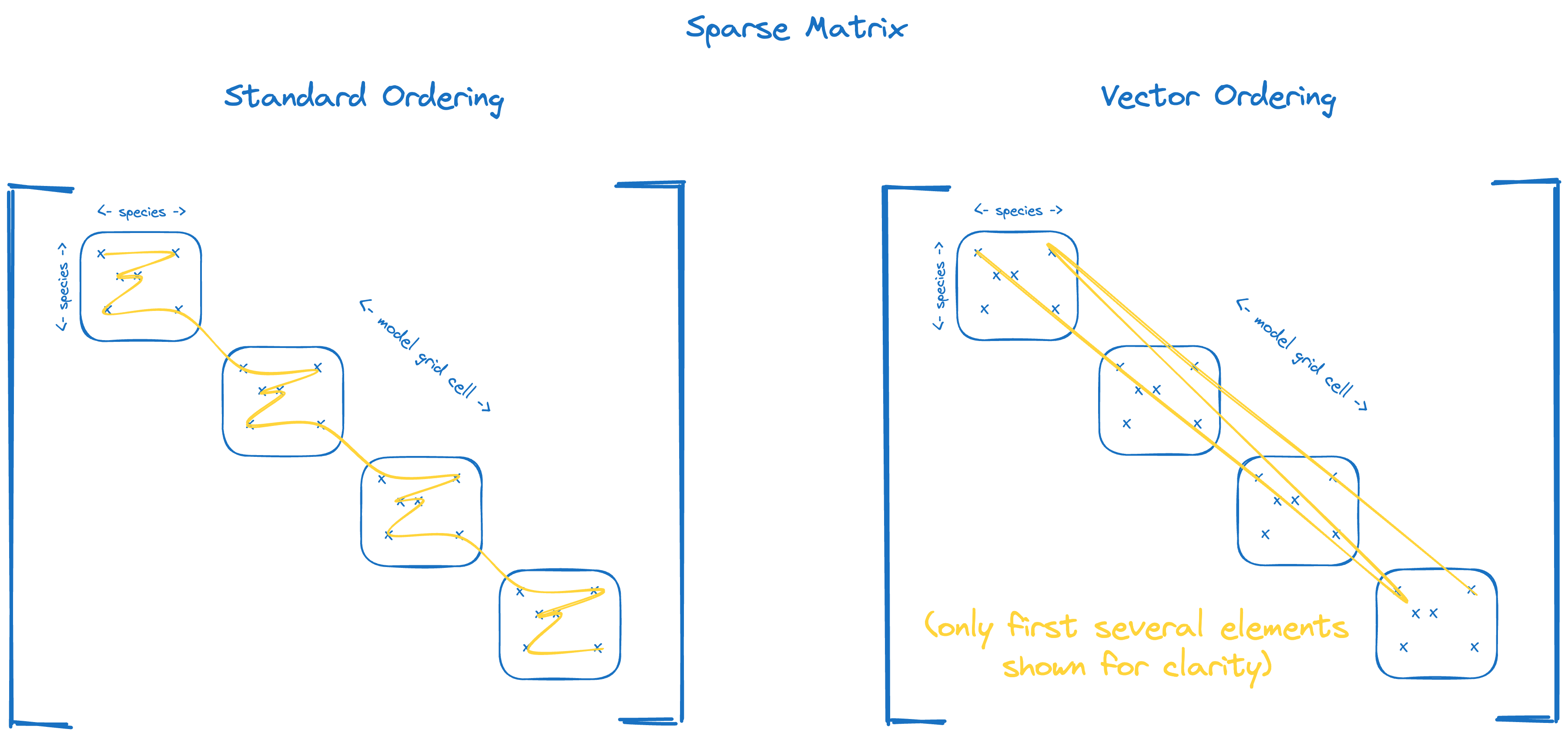
Element ordering for standard (left) and vector (right) ordered block-diagonal sparse matrices.#
micm::SparseMatrix, a sparse matrix data structureThe sparse matrix allows you to select the standard or vector ordering by applying a ordering policy to the
micm::SparseMatrixtype.
To demonstrate the effects of the ordering policy on sparse matrix objects, we create the same sparse matrix using each ordering policy:
    std::cout << std::endl;
  }

  micm::SparseMatrix<std::string> sparse_matrix{ micm::SparseMatrix<std::string>::Create(4)
                                                     .WithElement(0, 1)
                                                     .WithElement(2, 1)
                                                     .WithElement(2, 3)
                                                     .WithElement(3, 2)
                                                     .SetNumberOfBlocks(3) };

  micm::SparseMatrix<std::string, micm::SparseMatrixVectorOrdering<3>> sparse_vector_matrix{
    micm::SparseMatrix<std::string, micm::SparseMatrixVectorOrdering<3>>::Create(4)
        .WithElement(0, 1)
        .WithElement(2, 1)
        .WithElement(2, 3)
        .WithElement(3, 2)
Standard ordering is the default, and thus does not have to be specified as a template parameter.
When creating vector-ordered matrices, specify the second template argument using
micm::SparseMatrixVectorOrdering<L> where L is the number of blocks (i.e. grid cells) in the
block diagonal matrix.
Just like the dense matrix, the square bracket notation is always used as matrix[block][column][row].
We use this syntax to set the same values for each element of our two sparse matrices.
We created matrices of strings so the values can be set as block.column.row:
  micm::SparseMatrix<std::string, micm::SparseMatrixVectorOrdering<3>> sparse_vector_matrix{
    micm::SparseMatrix<std::string, micm::SparseMatrixVectorOrdering<3>>::Create(4)
        .WithElement(0, 1)
        .WithElement(2, 1)
        .WithElement(2, 3)
        .WithElement(3, 2)
        .SetNumberOfBlocks(3)
  };

  sparse_matrix[0][0][1] = sparse_vector_matrix[0][0][1] = "0.0.1";
  sparse_matrix[0][2][1] = sparse_vector_matrix[0][2][1] = "0.2.1";
  sparse_matrix[0][2][3] = sparse_vector_matrix[0][2][3] = "0.2.3";
  sparse_matrix[0][3][2] = sparse_vector_matrix[0][3][2] = "0.3.2";
  sparse_matrix[1][0][1] = sparse_vector_matrix[1][0][1] = "1.0.1";
  sparse_matrix[1][2][1] = sparse_vector_matrix[1][2][1] = "1.2.1";
We can again see the effects of the ordering policy by accessing the underlying data vector directly:
  sparse_matrix[1][3][2] = sparse_vector_matrix[1][3][2] = "1.3.2";
  sparse_matrix[2][0][1] = sparse_vector_matrix[2][0][1] = "2.0.1";
  sparse_matrix[2][2][1] = sparse_vector_matrix[2][2][1] = "2.2.1";
  sparse_matrix[2][2][3] = sparse_vector_matrix[2][2][3] = "2.2.3";
  sparse_matrix[2][3][2] = sparse_vector_matrix[2][3][2] = "2.3.2";

  std::cout << std::endl << "Sparse matrix standard ordering elements" << std::endl;
  for (auto& elem : sparse_matrix.AsVector())
  {
    std::cout << elem << std::endl;
  }
  std::cout << std::endl << "Sparse matrix vector ordering elements" << std::endl;
  for (auto& elem : sparse_vector_matrix.AsVector())
  {
    std::cout << elem << std::endl;
  }
}
Sparse matrix standard ordering elements
0.0.1
0.2.1
0.2.3
0.3.2
1.0.1
1.2.1
1.2.3
1.3.2
2.0.1
2.2.1
2.2.3
2.3.2

Sparse matrix vector ordering elements
0.0.1
1.0.1
2.0.1
0.2.1
1.2.1
2.2.1
0.2.3
1.2.3
2.2.3
0.3.2
1.3.2
2.3.2