Loading A Custom Box Model in MusicBox#

MusicBox has two primary ways of loading custom box models, being:

from a pre-made example configuration path, and
from your own JSON file.

Both of these will be looked at in this tutorial. Note: These configuration files will cover every aspect of the box model, being the initial and evolving conditions, the box model configurations, as well as the mechanism containing the species, reactions, and phases.

1. Loading Pre-made Box Model Examples#

MusicBox has a couple of built in examples that are formatted as JSON files through the Examples class. These are accessed through the path attribute in each example. Once accessed, it can be loaded into the box model through the loadJson() function, which takes in the path as a parameter. The supported examples include:

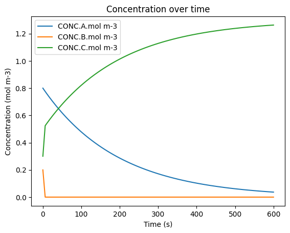
This code features the Analytical example, but feel free to test any of them by switching out the name where Analytical is in Examples.Analytical.path. To load, run, and visualize an example box model:

[1]:

from acom_music_box import MusicBox, Examples
import matplotlib.pyplot as plt
import logging
import sys

logging.disable(sys.maxsize) # Prevents log spam when running this cell

box_model = MusicBox()
conditions_path = Examples.Analytical.path
box_model.loadJson(conditions_path)
df = box_model.solve()
display(df)
df.plot(x='time.s', y=['CONC.A.mol m-3', 'CONC.B.mol m-3', 'CONC.C.mol m-3'], title='Concentration over time', ylabel='Concentration (mol m-3)', xlabel='Time (s)')
plt.show()

	time.s	ENV.temperature.K	ENV.pressure.Pa	ENV.air number density.mol m-3	CONC.A.mol m-3	CONC.B.mol m-3	CONC.C.mol m-3
0	0.0	200.0	70000.0	42.095324	0.800000	2.000000e-01	0.300000
1	6.0	200.0	70000.0	42.095324	0.775723	3.979221e-08	0.524277
2	12.0	200.0	70000.0	42.095324	0.752182	3.858465e-08	0.547818
3	18.0	200.0	70000.0	42.095324	0.729356	3.741374e-08	0.570644
4	24.0	200.0	70000.0	42.095324	0.707222	3.627836e-08	0.592777
...	...	...	...	...	...	...	...
96	576.0	200.0	70000.0	42.095324	0.041522	2.129939e-09	1.258478
97	582.0	200.0	70000.0	42.095324	0.040262	2.065302e-09	1.259738
98	588.0	200.0	70000.0	42.095324	0.039040	2.002627e-09	1.260960
99	594.0	200.0	70000.0	42.095324	0.037855	1.941854e-09	1.262145
100	600.0	200.0	70000.0	42.095324	0.036706	1.882926e-09	1.263294

101 rows × 7 columns

2. Loading a Custom JSON Box Model Configuration#

Loading your own JSON file is incredibly similar to loading a pre-made example, you just provide a path to your own configuration rather than an instance of the Examples class. To do so with a file called custom_box_model.json in the config subfolder:

[2]:

from acom_music_box import MusicBox
import matplotlib.pyplot as plt
import logging
import sys

logging.disable(sys.maxsize) # Prevents log spam when running this cell

box_model = MusicBox()
conditions_path = "config/custom_box_model.json"
box_model.loadJson(conditions_path)
df = box_model.solve()
display(df)
df.plot(x='time.s', y=['CONC.A.mol m-3', 'CONC.B.mol m-3', 'CONC.C.mol m-3'], title='Concentration over time', ylabel='Concentration (mol m-3)', xlabel='Time (s)')
plt.show()

Simulation Progress:   0%|          | 0/600.0 [00:00<?, ? [model integration steps (2.0 s)]/s]

	time.s	ENV.temperature.K	ENV.pressure.Pa	ENV.air number density.mol m-3	CONC.A.mol m-3	CONC.B.mol m-3	CONC.C.mol m-3
0	0.0	200.0	70000.0	42.095324	0.800000	2.000000e-01	0.300000
1	6.0	200.0	70000.0	42.095324	0.775723	3.979221e-08	0.524277
2	12.0	200.0	70000.0	42.095324	0.752182	3.858465e-08	0.547818
3	18.0	200.0	70000.0	42.095324	0.729356	3.741374e-08	0.570644
4	24.0	200.0	70000.0	42.095324	0.707222	3.627836e-08	0.592777
...	...	...	...	...	...	...	...
96	576.0	200.0	70000.0	42.095324	0.041522	2.129939e-09	1.258478
97	582.0	200.0	70000.0	42.095324	0.040262	2.065302e-09	1.259738
98	588.0	200.0	70000.0	42.095324	0.039040	2.002627e-09	1.260960
99	594.0	200.0	70000.0	42.095324	0.037855	1.941854e-09	1.262145
100	600.0	200.0	70000.0	42.095324	0.036706	1.882926e-09	1.263294

101 rows × 7 columns