GMST from AWS CMIP6 data

from matplotlib import pyplot as plt
import xarray as xr
import numpy as np
from dask.diagnostics import progress
from tqdm.autonotebook import tqdm
import intake
import fsspec
import seaborn as sns
import aiohttp
import dask
from dask.distributed import LocalCluster
import pelicanfs 
import os
from pelicanfs.core import OSDFFileSystem,PelicanMap 

#
gdex_url    =  'https://data.gdex.ucar.edu/'
cat_url     = gdex_url +  'd850001/catalogs/osdf/cmip6-aws/cmip6-osdf-zarr.json'

cluster = LocalCluster()
client = cluster.get_client()

# Scale the local cluster
n_workers = 5
cluster.scale(n_workers)
cluster

col = intake.open_esm_datastore(cat_url)
col

[eid for eid in col.df['experiment_id'].unique() if 'ssp' in eid]

# there is currently a significant amount of data for these runs
expts = ['historical', 'ssp245', 'ssp370']

query = dict(
    experiment_id=expts,
    table_id='Amon',
    variable_id=['tas'],
    member_id = 'r1i1p1f1',
    #activity_id = 'CMIP',
)

col_subset = col.search(require_all_on=["source_id"], **query)
col_subset

col_subset.df.groupby("source_id")[["experiment_id", "variable_id", "table_id","activity_id"]].nunique()

col_subset.df

# %%time
# dsets_osdf  = col_subset.to_dataset_dict()
# print(f"\nDataset dictionary keys:\n {dsets_osdf.keys()}")

def drop_all_bounds(ds):
    drop_vars = [vname for vname in ds.coords
                 if (('_bounds') in vname ) or ('_bnds') in vname]
    return ds.drop_vars(drop_vars)

def open_dset(df):
    assert len(df) == 1
    mapper = fsspec.get_mapper(df.zstore.values[0])
    path = df.zstore.values[0][7:]+".zmetadata"
    ds = xr.open_zarr(mapper, consolidated=True,zarr_format=2) #You can skip the zarr_ormat option if you have zarr version 2
    a_data = mapper.fs.get_access_data()
    responses = a_data.get_responses(path)
    print(responses)
    return drop_all_bounds(ds)

def open_delayed(df):
    return dask.delayed(open_dset)(df)

from collections import defaultdict
dsets = defaultdict(dict)

for group, df in col_subset.df.groupby(by=['source_id', 'experiment_id']):
    dsets[group[0]][group[1]] = open_delayed(df)

dsets_ = dask.compute(dict(dsets))[0]

#calculate global means
def get_lat_name(ds):
    for lat_name in ['lat', 'latitude']:
        if lat_name in ds.coords:
            return lat_name
    raise RuntimeError("Couldn't find a latitude coordinate")

def global_mean(ds):
    lat = ds[get_lat_name(ds)]
    weight = np.cos(np.deg2rad(lat))
    weight /= weight.mean()
    other_dims = set(ds.dims) - {'time'}
    return (ds * weight).mean(other_dims)

expt_da = xr.DataArray(expts, dims='experiment_id', name='experiment_id',
                       coords={'experiment_id': expts})

dsets_aligned = {}

for k, v in tqdm(dsets_.items()):
    expt_dsets = v.values()
    if any([d is None for d in expt_dsets]):
        print(f"Missing experiment for {k}")
        continue

    for ds in expt_dsets:
        ds.coords['year'] = ds.time.dt.year

    # workaround for
    # https://github.com/pydata/xarray/issues/2237#issuecomment-620961663
    dsets_ann_mean = [v[expt].pipe(global_mean).swap_dims({'time': 'year'})
                             .drop_vars('time').coarsen(year=12).mean()
                      for expt in expts]

    # align everything with the 4xCO2 experiment
    dsets_aligned[k] = xr.concat(dsets_ann_mean, join='outer',dim=expt_da)

%%time
with progress.ProgressBar():
    dsets_aligned_ = dask.compute(dsets_aligned)[0]

source_ids = list(dsets_aligned_.keys())
source_da = xr.DataArray(source_ids, dims='source_id', name='source_id',
                         coords={'source_id': source_ids})

big_ds = xr.concat([ds.reset_coords(drop=True)
                    for ds in dsets_aligned_.values()],
                    dim=source_da)

big_ds

osdf_fs = OSDFFileSystem()
print(osdf_fs)
#
obs_url    = '/ncar/gdex/d850001/HadCRUT.5.0.2.0.analysis.summary_series.global.monthly.nc'
#
obs_ds = xr.open_dataset(osdf_fs.open(obs_url,mode='rb'),engine='h5netcdf').tas_mean
obs_ds

# Compute annual mean temperatures anomalies
obs_gmsta = obs_ds.resample(time='YS').mean(dim='time')
obs_gmsta

df_all = big_ds.to_dataframe().reset_index()
df_all.head()

# Compute anomaly w.r.t 1960-1990 baseline
# Define the baseline period
baseline_df = df_all[(df_all["year"] >= 1960) & (df_all["year"] <= 1990)]

# Compute the baseline mean
baseline_mean = baseline_df["tas"].mean()

# Compute anomalies
df_all["tas_anomaly"] = df_all["tas"] - baseline_mean
df_all

obs_df = obs_gmsta.to_dataframe(name='tas_anomaly').reset_index()
# obs_df

# Convert 'time' to 'year' (keeping only the year)
obs_df['year'] = obs_df['time'].dt.year

# Drop the original 'time' column since we extracted 'year'
obs_df = obs_df[['year', 'tas_anomaly']]
obs_df

# Create the main plot
g = sns.relplot(data=df_all, x="year", y="tas_anomaly",
                hue='experiment_id', kind="line", errorbar="sd", aspect=2, palette="Set2")  # Adjust the color palette)

# Get the current axis from the FacetGrid
ax = g.ax

# Overlay the observational data in red
sns.lineplot(data=obs_df, x="year", y="tas_anomaly",color="red", 
             linestyle="dashed", linewidth=2,label="Observations", ax=ax)

# Adjust the legend to include observations
ax.legend(title="Experiment ID + Observations")

# Show the plot
plt.show()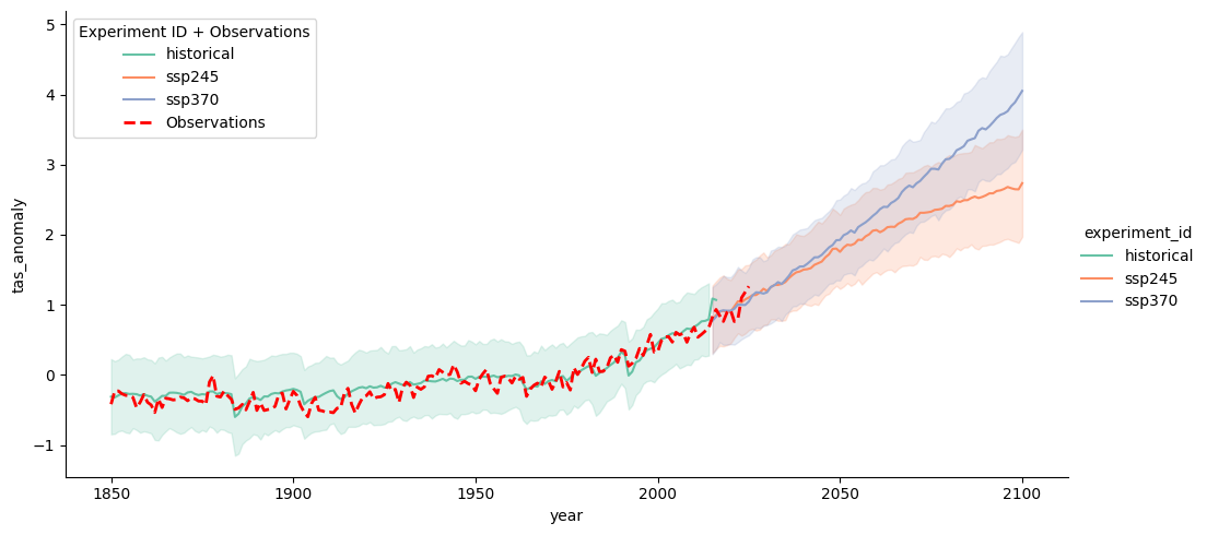

# cluster.close()

# sns.relplot(data=df_all,x="year", y="tas_anomaly", hue='experiment_id',kind="line", errorbar="sd", aspect=2)