JJA precipitation across South America (SAAG)

origin:ncar-posix platform:casper dataset:saag task:visualization level:intermediate

This notebook illustrates how to make diagnostic plots using the WRF-SAAG dataset hosted on NCAR’s Geoscience Data Exchange (GDEX).

WRF-SAAG is a 4-km, hourly, ~22-year convection-permitting simulation of the current climate over South America, produced by NCAR’s Research Applications Laboratory and the South America Affinity Group by dynamically downscaling ERA5 with the Weather Research and Forecasting (WRF) model. The historical run spans January 2000 – December 2021 and is described in Domínguez et al. (2024, BAMS).

The native data are hourly NetCDF files — roughly 190,000 files for the full record — which would be awkward to stream individually. GDEX provides a kerchunk reference layer on top of those NetCDFs that exposes the entire archive as a single virtual xarray.Dataset. With it, we can slice the 22-year hourly record with a single xarray call and only stream the bytes we actually need.

What this notebook does¶

For one calendar year (2020) we produce a 3-panel map of monthly precipitation totals for the austral winter (June–July–August) over South America. We focus on a single year and season so the workflow stays tractable while still showing the continent’s strong regional precipitation contrasts.

# Imports
import os
import calendar
import numpy as np
import xarray as xr
import matplotlib.pyplot as plt
import cartopy.crs as ccrs
import cartopy.feature as cfeature
from matplotlib.colors import ListedColormap, BoundaryNorm

# Dask
from dask_jobqueue import PBSCluster
from dask.distributed import Client

# GDEX kerchunk reference for the SAAG 2D (surface) variables, served over HTTPS
kerchunk_url = "https://data.gdex.ucar.edu/d616000/kerchunk/wrf2d-remote-osdf.parq"
print(kerchunk_url)

https://data.gdex.ucar.edu/d616000/kerchunk/wrf2d-remote-osdf.parq

# Set up your scratch folder path
username       = os.environ["USER"]
glade_scratch  = "/glade/derecho/scratch/" + username
print(glade_scratch)

/glade/derecho/scratch/harshah

Create a PBS cluster¶

# Create a PBS cluster.
# Each worker must hold the ~5 GB SAAG kerchunk reference in memory, so we use a
# handful of larger-memory (8 GiB) workers rather than many small ones.
cluster = PBSCluster(
    job_name        = "saag-precip",
    cores           = 1,
    memory          = "8GiB",
    processes       = 1,
    local_directory = f"{glade_scratch}/dask/spill/",
    log_directory   = f"{glade_scratch}/dask/logs/",
    resource_spec   = "select=1:ncpus=1:mem=8GB",
    queue           = "casper",
    walltime        = "1:00:00",
    interface       = "ext",)

# Scale the cluster and display the dashboard link
n_workers = 5
client = Client(cluster)
cluster.scale(n_workers)
client.wait_for_workers(n_workers=n_workers)
cluster

/glade/u/home/harshah/.conda/envs/osdf/lib/python3.11/site-packages/distributed/node.py:187: UserWarning: Port 8787 is already in use.
Perhaps you already have a cluster running?
Hosting the HTTP server on port 39403 instead
  warnings.warn(

Load SAAG data from GDEX using kerchunk reference files¶

Find the precipitation variable¶

Choosing how to access SAAG¶

SAAG is published as hourly NetCDF files — roughly 190,000 files for the full 2000–2021 record. Streaming that many small files individually would be slow and brittle.

GDEX adds a kerchunk reference layer on top of those NetCDFs. A kerchunk reference is a parquet file that records which byte range of which NetCDF holds each chunk. From the reader’s perspective it looks like a single virtual xarray.Dataset, and you only stream the bytes you actually request.

GDEX publishes two such references for SAAG, each aggregating across all years and all variables in its group:

File	Coverage
`wrf2d-remote-https.parq`	All 2D (surface) variables — precipitation, 2-m temperature, surface fluxes, …
`wrf3d-remote-https.parq`	All 3D variables — temperature, humidity, wind on model levels

We want hourly precipitation (PREC_ACC_NC), a 2D variable, so we open the wrf2d reference with xarray’s kerchunk engine. The result is the full ~22-year hourly record of every 2D variable in a single Dataset — ready to slice with .sel(Time=...).

Load data into xarray¶

%%time
# One kerchunk reference exposes the full ~22-year hourly 2D archive.
# The first open takes ~30-60 s while kerchunk parses the parquet index;
# subsequent slicing is lazy and fast.
ds = xr.open_dataset(kerchunk_url, engine="kerchunk")

pr    = ds["PREC_ACC_NC"]          # (Time: 192889, south_north: 2027, west_east: 1471)
lat2d = ds["XLAT"].isel(Time=0)    # 2D static lat/lon for plotting + masking
lon2d = ds["XLONG"].isel(Time=0)
pr

/glade/u/home/harshah/.conda/envs/osdf/lib/python3.11/site-packages/tqdm/auto.py:21: TqdmWarning: IProgress not found. Please update jupyter and ipywidgets. See https://ipywidgets.readthedocs.io/en/stable/user_install.html
  from .autonotebook import tqdm as notebook_tqdm

CPU times: user 10.8 s, sys: 3.14 s, total: 14 s
Wall time: 15.8 s

Data Analysis¶

Monthly precipitation for austral winter (JJA)¶

We sum hourly precipitation to monthly totals for June, July, and August of 2020 and lay them out as a 3-panel map. June–August is the dry season over much of tropical South America but the wet season along the northern coast and the southern Andes, so the panels highlight the continent’s strong regional contrasts.

Compute the seasonal totals¶

The next cell streams hourly precipitation from GDEX for June, July, and August 2020 and reduces each month to a single grid.

%%time
# JJA (Jun-Aug) 2020 precipitation: reduce ONE month at a time (memory-safe),
# keeping the three monthly grids in a list for the 3-panel plot below.
pr_2020 = pr.sel(Time="2020")

jja = []
for m in (6, 7, 8):
    # retries=2 lets Dask re-fetch chunks that transiently fail with
    # ReferenceNotReachable under the high request volume of a full-month
    # hourly reduction (the kerchunk targets are valid; see conus404).
    pr_m = pr_2020.sel(Time=pr_2020["Time"].dt.month == m).sum("Time").compute(retries=2)
    jja.append(pr_m)
    print(f"month {m:2d} done")

month  6 done
month  7 done
month  8 done
CPU times: user 47.6 s, sys: 4.89 s, total: 52.5 s
Wall time: 19min 41s

%%time
proj  = ccrs.PlateCarree()
trans = ccrs.PlateCarree()

# Stack the three monthly grids (June, July, August) into a 'month' dimension
pr_months = xr.concat(jja, dim="month").assign_coords(month=[6, 7, 8])

# Discrete colormap based on the NCL precip3_16lev palette (RGB 0-255)
_rgb255 = [
    (255,255,255), (214,226,255), (181,201,255), (142,178,255),
    (127,150,255), (114,133,248), ( 99,112,248), (  0,158, 30),
    ( 60,188, 61), (179,209,110), (185,249,110), (255,249, 19),
    (255,163,  9), (229,  0,  0), (189,  0, 31), (165,  0, 33),
]
cmap_pr = ListedColormap(np.array(_rgb255) / 255, name="precip3_16lev")
levels  = np.arange(0, 301, 20)        # 0-300 mm monthly total (16 boundaries)
norm    = BoundaryNorm(levels, ncolors=cmap_pr.N, extend="max")

# Coarsen 4x for plotting only (saves cartopy memory)
COARSEN  = 4
pr_plot  = pr_months.coarsen(south_north=COARSEN, west_east=COARSEN, boundary="trim").mean()
lat_plot = lat2d.coarsen(south_north=COARSEN, west_east=COARSEN, boundary="trim").mean()
lon_plot = lon2d.coarsen(south_north=COARSEN, west_east=COARSEN, boundary="trim").mean()

fig, axes = plt.subplots(
    1, 3, figsize=(15, 5.5),
    subplot_kw={"projection": proj},
    constrained_layout=True,
)

for i, ax in enumerate(axes):
    month_int = int(pr_plot.month.values[i])
    im = ax.pcolormesh(
        lon_plot.values, lat_plot.values, pr_plot.isel(month=i).values,
        transform=trans, cmap=cmap_pr, norm=norm, shading="auto",
    )
    ax.add_feature(cfeature.COASTLINE, lw=0.5)
    ax.add_feature(cfeature.BORDERS, lw=0.4)
    ax.add_feature(cfeature.STATES, lw=0.15)
    ax.set_extent([-93, -20, -56, 16], crs=trans)
    ax.set_title(calendar.month_name[month_int], fontsize=12)

cbar = fig.colorbar(
    im, ax=axes, shrink=0.6, orientation="vertical",
    ticks=levels, extend="max",
    label="Monthly precipitation (mm)",
)
fig.suptitle("SAAG monthly precipitation — JJA 2020", fontsize=14, y=1.02)
plt.show()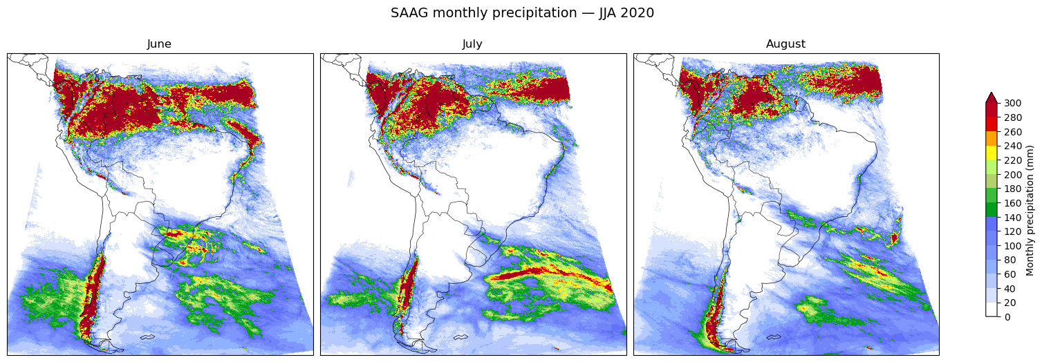

CPU times: user 3.79 s, sys: 516 ms, total: 4.31 s
Wall time: 11 s

cluster.close()

Summary¶

We accessed the WRF-SAAG convection-permitting simulation of South America through GDEX’s kerchunk reference layer, sliced the 2020 austral-winter months from the ~22-year hourly archive, and reduced June, July, and August each to a monthly precipitation total — shown as a 3-panel map. June–August is the dry season across much of tropical South America but the wet season along the northern coast and the southern Andes, and the panels capture those contrasts.

To build a precipitation climatology rather than a single year, repeat the monthly reduction over many years and average.

References¶

Dominguez, F., Rasmussen, R., Liu, C., Ikeda, K., Prein, A., Varble, A., Arias, P. A., Bacmeister, J., Bettolli, M. L., Callaghan, P., Carvalho, L. M. V., Castro, C. L., Chen, F., Chug, D., Chun, K. P. (Sun), Dai, A., Danaila, L., da Rocha, R. P., Nascimento, E. de L., … Schneider, T. (2024). Advancing South American Water and Climate Science through Multidecadal Convection-Permitting Modeling. Bulletin of the American Meteorological Society, 105(1), E32–E44. 10.1175/bams-d-22-0226.1