Access CMIP6 zarr data from AWS using the osdf protocol and compute different precipitation statistics
- This workflow is an adaptation of https://
gallery .pangeo .io /repos /pangeo -gallery /cmip6 /precip _frequency _change .html - Also see, the paper Pendergrass & Deser (2017)
- And the article https://
climatedataguide .ucar .edu /climate -data /gpcp -daily -global -precipitation -climatology -project which inspired the workflow
Table of Contents
Section 1: Introduction
- Load python packkages
- Load catalog url
from matplotlib import pyplot as plt
import xarray as xr
import numpy as np
import dask
from dask.diagnostics import progress
from tqdm.autonotebook import tqdm
import intake
import fsspec
import seaborn as sns
import re
import aiohttp
from dask_jobqueue import PBSCluster
import pandas as pd
from xhistogram.xarray import histogram
/glade/derecho/scratch/harshah/tmp/ipykernel_37992/3451259092.py:6: TqdmExperimentalWarning: Using `tqdm.autonotebook.tqdm` in notebook mode. Use `tqdm.tqdm` instead to force console mode (e.g. in jupyter console)
from tqdm.autonotebook import tqdm
# import fsspec.implementations.http as fshttp
from pelicanfs.core import OSDFFileSystem,PelicanMap
lustre_scratch = "/lustre/desc1/scratch/harshah"
#
gdex_url = 'https://data.gdex.ucar.edu/'
# cat_url = gdex_url + 'd850001/catalogs/osdf/cmip6-aws/cmip6-osdf-zarr.json'
cat_url = 'https://cmip6-pds.s3.amazonaws.com/pangeo-cmip6.json'Section 2: Select Dask Cluster
Select the Dask cluster type
The default will be LocalCluster as that can run on any system.
If running on a HPC computer with a PBS Scheduler, set to True. Otherwise, set to False.
USE_PBS_SCHEDULER = TrueIf running on Jupyter server with Dask Gateway configured, set to True. Otherwise, set to False.
USE_DASK_GATEWAY = FalsePython function for a PBS cluster
# Create a PBS cluster object
def get_pbs_cluster():
    """ Create cluster through dask_jobqueue.
    """
    from dask_jobqueue import PBSCluster
    cluster = PBSCluster(
        job_name = 'dask-osdf-24',
        cores = 1,
        memory = '4GiB',
        processes = 1,
        local_directory = lustre_scratch + '/dask/spill',
        log_directory = lustre_scratch + '/dask/logs/',
        resource_spec = 'select=1:ncpus=1:mem=4GB',
        queue = 'casper',
        walltime = '3:00:00',
        #interface = 'ib0'
        interface = 'ext'
    )
    return cluster
Python function for a Gateway Cluster
def get_gateway_cluster():
    """ Create cluster through dask_gateway
    """
    from dask_gateway import Gateway

    gateway = Gateway()
    cluster = gateway.new_cluster()
    cluster.adapt(minimum=2, maximum=4)
    return cluster
def get_local_cluster():
""" Create cluster using the Jupyter server's resources
"""
from distributed import LocalCluster, performance_report
cluster = LocalCluster()
cluster.scale(6)
return clusterPython logic for a Local Cluster
This uses True/False boolean logic based on the variables set in the previous cells
# Obtain dask cluster in one of three ways
if USE_PBS_SCHEDULER:
    cluster = get_pbs_cluster()
elif USE_DASK_GATEWAY:
    cluster = get_gateway_cluster()
else:
    cluster = get_local_cluster()

# Connect to cluster
from distributed import Client
client = Client(cluster)
# Scale the cluster and display cluster dashboard URL
n_workers =8
cluster.scale(n_workers)
client.wait_for_workers(n_workers = n_workers)
clusterLoading...
Section 3: Data Loading
- Load catalog and select data subset
col = intake.open_esm_datastore(cat_url)
col
Loading...
[eid for eid in col.df['experiment_id'].unique() if 'ssp' in eid]['esm-ssp585-ssp126Lu',
'ssp126-ssp370Lu',
'ssp370-ssp126Lu',
'ssp585',
'ssp245',
'ssp370-lowNTCF',
'ssp370SST-ssp126Lu',
'ssp370SST',
'ssp370pdSST',
'ssp370SST-lowCH4',
'ssp370SST-lowNTCF',
'ssp126',
'ssp119',
'ssp370',
'esm-ssp585',
'ssp245-nat',
'ssp245-GHG',
'ssp460',
'ssp434',
'ssp534-over',
'ssp245-aer',
'ssp245-stratO3',
'ssp245-cov-fossil',
'ssp245-cov-modgreen',
'ssp245-cov-strgreen',
'ssp245-covid',
'ssp585-bgc']# there is currently a significant amount of data for these runs
expts = ['historical', 'ssp585']
query = dict(
experiment_id=expts,
table_id='3hr',
variable_id=['pr'],
#member_id = 'r1i1p1f1',
#activity_id = 'CMIP',
)
col_subset = col.search(require_all_on=["source_id"], **query)
col_subsetLoading...
col_subset.df.groupby("source_id")[["experiment_id", "variable_id", "table_id","activity_id"]].nunique()Loading...
col_subset.dfLoading...
source_ids = col_subset.df['source_id'].unique()
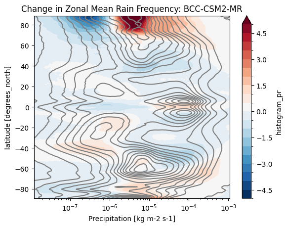
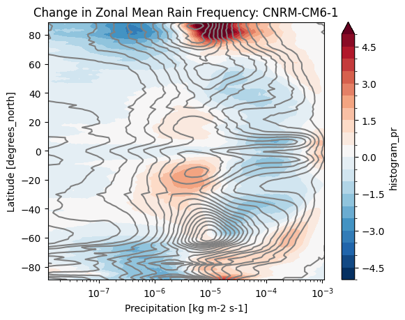
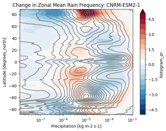
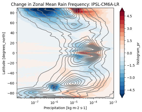
source_idsarray(['BCC-CSM2-MR', 'CNRM-CM6-1', 'CNRM-ESM2-1', 'IPSL-CM6A-LR'],
dtype=object)# %%time
# dsets_osdf = col_subset.to_dataset_dict()
# print(f"\nDataset dictionary keys:\n {dsets_osdf.keys()}")def load_pr_data(source_id, expt_id):
"""
Load 3hr precip data for given source and expt ids
"""
df_subset = col_subset.df
uri = df_subset[(df_subset.source_id == source_id) &
(df_subset.experiment_id == expt_id)].zstore.values[0]
ds = xr.open_zarr(fsspec.get_mapper(uri,anon=True), consolidated=True)
return dsdef precip_hist(ds, nbins=100, pr_log_min=-3, pr_log_max=2):
"""
Calculate precipitation histogram for a single model.
Lazy.
"""
assert ds.pr.units == 'kg m-2 s-1'
# mm/day
bins_mm_day = np.hstack([[0], np.logspace(pr_log_min, pr_log_max, nbins)])
bins_kg_m2s = bins_mm_day / (24*60*60)
pr_hist = histogram(ds.pr, bins=[bins_kg_m2s], dim=['lon']).mean(dim='time')
log_bin_spacing = np.diff(np.log(bins_kg_m2s[1:3])).item()
pr_hist_norm = 100 * pr_hist / ds.sizes['lon'] / log_bin_spacing
pr_hist_norm.attrs.update({'long_name': 'zonal mean rain frequency',
'units': '%/Δln(r)'})
return pr_hist_norm
def precip_hist_for_expts(dsets, experiment_ids):
"""
Calculate histogram for a suite of experiments.
Eager.
"""
# actual data loading and computations happen in this next line
pr_hists = [precip_hist(ds).load() for ds in [ds_hist, ds_ssp]]
pr_hist = xr.concat(pr_hists, dim=xr.Variable('experiment_id', experiment_ids))
return pr_hist%%time
results = {}
for source_id in tqdm(source_ids):
# get a 20 year period
ds_hist = load_pr_data(source_id, 'historical').sel(time=slice('1980', '2000'))
ds_ssp = load_pr_data(source_id, 'ssp585').sel(time=slice('2080', '2100'))
print(ds_hist)
pr_hist = precip_hist_for_expts([ds_hist, ds_ssp], expts)
results[source_id] = pr_histLoading...
Section 4: Data Analysis
- Calculate precipitation statistics
- Grab some observations ?
- Plot precipitation changes for different CMIP6 models
def plot_precip_changes(pr_hist, vmax=5):
    """
    Visualize the output
    """
    pr_hist_diff = (pr_hist.sel(experiment_id='ssp585') -
                    pr_hist.sel(experiment_id='historical'))
    pr_hist.sel(experiment_id='historical')[:, 1:].plot.contour(xscale='log', colors='0.5', levels=21)
    pr_hist_diff[:, 1:].plot.contourf(xscale='log', vmax=vmax, levels=21)
%%time
title = 'Change in Zonal Mean Rain Frequency'
for source_id, pr_hist in results.items():
plt.figure()
plot_precip_changes(pr_hist)
plt.title(f'{title}: {source_id}')CPU times: user 161 ms, sys: 9.99 ms, total: 171 ms
Wall time: 177 ms
cluster.close()- Pendergrass, A. G., & Deser, C. (2017). Climatological Characteristics of Typical Daily Precipitation. Journal of Climate, 30(15), 5985–6003. 10.1175/jcli-d-16-0684.1