Access CESM2 data from RDA and compute climatology average

# Imports
import geocat.comp as gc
import intake
import numpy as np
import pandas as pd
import xarray as xr
# import seaborn as sns
import re
import aiohttp

import fsspec.implementations.http as fshttp
from pelicanfs.core import PelicanFileSystem, PelicanMap, OSDFFileSystem

import dask 
from dask_jobqueue import PBSCluster
from dask.distributed import Client
from dask.distributed import performance_report

year0  = '1991'
year1  = '2020'
year0_str = str(year0)
year1_str = str(year1)

#Boulder coordinates
boulder_lat = 40.0150 
boulder_lon = (360-105.2705)%360
print(boulder_lat,boulder_lon)

40.015 254.7295

# File paths
rda_scratch = '/gpfs/csfs1/collections/rda/scratch/harshah'
# catalog_url = 'https://data.rda.ucar.edu/d010092/catalogs/d010092-posix-zarr.json' #Use this if you are working on NCAR's Casper
catalog_url = 'https://data.rda.ucar.edu/d010092/catalogs/d010092-osdf-zarr.json'

Spin up a cluster¶

# Create a PBS cluster object
cluster = PBSCluster(
    job_name = 'dask-wk24-hpc',
    cores = 1,
    memory = '4GiB',
    processes = 1,
    local_directory = rda_scratch+'/dask/spill',
    resource_spec = 'select=1:ncpus=1:mem=4GB',
    queue = 'casper',
    walltime = '3:00:00',
    log_directory = rda_scratch+'/dask/logs',
    #interface = 'ib0'
    interface = 'ext'
)

client = Client(cluster)
client

cluster.scale(2)
cluster

Load CESM2 temperature data and apply geocat-comp’s climatology average¶

osdf_catalog = intake.open_esm_datastore(catalog_url)
osdf_catalog

osdf_catalog.df['path'].head().values

array(['osdf:///ncar/rda/d010092/atm/daily/cesm2LE-historical-cmip6-FLNS.zarr',
       'osdf:///ncar/rda/d010092/atm/daily/cesm2LE-historical-cmip6-FLNSC.zarr',
       'osdf:///ncar/rda/d010092/atm/daily/cesm2LE-historical-cmip6-FLUT.zarr',
       'osdf:///ncar/rda/d010092/atm/daily/cesm2LE-historical-cmip6-FSNS.zarr',
       'osdf:///ncar/rda/d010092/atm/daily/cesm2LE-historical-cmip6-FSNSC.zarr'],
      dtype=object)

osdf_catalog_temp = osdf_catalog.search(variable ='TREFHT', frequency ='daily',forcing_variant='cmip6')
osdf_catalog_temp

%%time
#dsets = osdf_catalog_temp.to_dataset_dict(storage_options={'anon':True})
dsets = osdf_catalog_temp.to_dataset_dict()

%%time
dsets.keys()

CPU times: user 3 μs, sys: 0 ns, total: 3 μs
Wall time: 4.05 μs

dict_keys(['atm.historical.daily.cmip6', 'atm.ssp370.daily.cmip6'])

historical_cmip6 = dsets['atm.historical.daily.cmip6']
historical_cmip6 = historical_cmip6.TREFHT
historical_cmip6

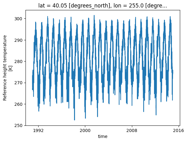
To illustrate how the function works select small subset¶

Choose data between year0 and year1
Choose data from only one member
Choose data for Boulder

%%time
historical_cmip6_30years = historical_cmip6.isel(member_id=0).sel(lat =boulder_lat,lon=boulder_lon,method='nearest').\
                             sel(time = slice(f'{year0_str}-01-01', f'{year1_str}-12-31'))
historical_cmip6_30years

%%time
# Plot raw data
historical_cmip6_30years.plot()

CPU times: user 14.7 s, sys: 730 ms, total: 15.4 s
Wall time: 5min 30s

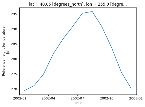
# historical_cmip6_30years.values

%%time
hist_cmip6_monthly = gc.climatology_average(historical_cmip6_30years,freq='month')
hist_cmip6_monthly

%%time
hist_cmip6_monthly.plot()

CPU times: user 568 ms, sys: 40.3 ms, total: 608 ms
Wall time: 11.5 s

cluster.close()