Access NOAA’s SONAR data hosted on AWS via OSDF protocol

For more information using the dataset, see https://cires.gitbook.io/ncei-wcsd-archive
This notebook is heavily inspried by the google colab notebook https://colab.research.google.com/drive/1-I56QOIftj9sewlbyzTzncdRt54Fh51d?usp=sharing#scrollTo=bCG81-1XOGqc
In this notebook, we will use the osdf protocol to access data from a zarr store via PelicanFS.
We will access the data using OSDF’s AWS open data origin.
For more details about pelicanfs, see https://github.com/PelicanPlatform/pelicanfs

Overview¶

The size and physiological characteristics of marine organisms determine their reflectance properties. An organisms backscatter also depends on the sonar frequency. Frequency differencing of the sonar’s volume backscattering strength (Sv) called “dB differencing” is a common analysis technique to help differentiate sources of acoustic scatterers.
This notebook demonstrates the use of frequency differencing on some Level 2 EK60 data.
The Level 2 data can be found here: https://noaa-wcsd-zarr-pds.s3.us-east-1.amazonaws.com/level_2/Bell_M._Shimada/SH1507/EK60/SH1507.zarr/
The files can be explored by navigating to the following AWS file explorer: https://noaa-wcsd-zarr-pds.s3.amazonaws.com/index.html#level_2/Bell_M._Shimada/SH1507/EK60/SH1507.zarr/

Import package, define parameters and functions¶

# Display output of plots directly in Notebook
import matplotlib.pyplot as plt
import warnings
warnings.filterwarnings("ignore")

import intake
import numpy as np
import pandas as pd
import xarray as xr
import s3fs
import seaborn as sns
import re
import nest_asyncio
nest_asyncio.apply()

from pelicanfs.core import PelicanFileSystem, PelicanMap,OSDFFileSystem 
import fsspec.implementations.http as fshttp

import dask 
from dask_jobqueue import PBSCluster
from dask.distributed import Client
from dask.distributed import performance_report

Use OSDF protocol to access data¶

Set up osdf url to use with PelicanFS¶

We should one of the two pelicanFS FSSpec protocols (‘osdf’ or ‘pelican’) instead of the https protocol.
So, the urls will look like: osdf_discovery_url + namespace prefix/aws_region/bucket_name/path to file or object
osdf_discovery_url = osdf:///, namespace_prefix = aws-opendata
aws_region = us-east-1, bucket_name = ‘noaa-wcsd-zarr-pds’
zarr_store = ‘level_2/Bell_M._Shimada/SH1507/EK60/SH1507.zarr’
An example url:
osdf:///us-east-1/aws-opendata/noaa-wcsd-zarr-pds/evel_2/Bell_M._Shimada/SH1507/EK60/SH1507.zarr

%%time
osdf_fs = OSDFFileSystem() # OSDFFileSystem is already aware of the osdf discovery url

CPU times: user 1.45 ms, sys: 0 ns, total: 1.45 ms
Wall time: 1.48 ms

%%time
# Compose url using s3 protocol
bucket_name = 'noaa-wcsd-zarr-pds'

ship_name   = 'Bell_M._Shimada'
cruise_name = 'SH1507'
sensor_name = 'EK60'

zarr_store = f'{cruise_name}.zarr'

# How an s3 path would look 
s3_zarr_store_path = f"{bucket_name}/level_2/{ship_name}/{cruise_name}/{sensor_name}/{zarr_store}"
print(s3_zarr_store_path)

noaa-wcsd-zarr-pds/level_2/Bell_M._Shimada/SH1507/EK60/SH1507.zarr
CPU times: user 54 μs, sys: 0 ns, total: 54 μs
Wall time: 56 μs

# Compose url using OSDF protocol
namespace_prefix = '/aws-opendata' #In this current version of pelfs, this slash is necessary
aws_region       = 'us-east-1'
osdf_path        = f"{namespace_prefix}/{aws_region}/{s3_zarr_store_path}"
print(osdf_path)

# This just prepends the osdf_disovery_url to the osdf_path
osdf_zarr_store_path = PelicanMap(osdf_path, osdf_fs)

/aws-opendata/us-east-1/noaa-wcsd-zarr-pds/level_2/Bell_M._Shimada/SH1507/EK60/SH1507.zarr

Opening a Zarr store with Xarray¶

We will open the S3 Zarr store using Xarray (the “consolidated” parameter just defines whether we are interested in reading the metadata in a consolidated manner, “None” is the desired value).

# %%time
# # First use s3
# s3_file_system = s3fs.S3FileSystem(anon=True)
# store          = s3fs.S3Map(root=s3_zarr_store_path, s3=s3_file_system, check=False)
# cruise         = xr.open_zarr(store=store, consolidated=None)

%%time
# Now use OSDF protocol: 
cruise_osdf = xr.open_zarr(osdf_zarr_store_path,consolidated = None)
cruise_osdf

Load data and plot echogram¶

Subsetting on one hour worth of data near an area of interest. We’ll define select_times from 19:00 to 20:00 on July 19th 2015.

# roughly covering the raw files from SaKe2015-D20150719-T193412.raw to SaKe2015-D20150719-T195842.raw
start_time = np.datetime64('2015-07-19T19:00:00')
end_time = np.datetime64('2015-07-19T20:00:00')

select_times = (cruise_osdf.time > start_time) & (cruise_osdf.time < end_time)

We can then use this slice of select_times to select the Sv values for the specific subset of time. Additional subsetting can also be added to the query, for example we can additionally subset by defining a selected frequency. The example below selects 18 kHz for the time interval of interest and store this in Sv_18 (drop=True means that the coordinate labels that do not meet the condition are not just masked but also dropped from the result)

Sv_38 = cruise_osdf.sel(frequency=38000).where((select_times), drop=True).Sv
print(Sv_38)

<xarray.DataArray 'Sv' (depth: 2800, time: 2959)> Size: 33MB
dask.array<where, shape=(2800, 2959), dtype=float32, chunksize=(512, 512), chunktype=numpy.ndarray>
Coordinates:
  * depth      (depth) float64 22kB nan 0.25 0.5 0.75 ... 699.5 699.8 700.0
    frequency  float32 4B 3.8e+04
  * time       (time) datetime64[ns] 24kB 2015-07-19T19:08:39.063712768 ... 2...
Attributes:
    long_name:  Volume backscattering strength (Sv re 1 m-1)
    units:      dB

%%time
Sv_38.dropna(dim='depth').plot(yincrease=False, cmap='jet', vmin=-80, vmax=-30)

plt.title(f"Sv 38 kHz")

CPU times: user 838 ms, sys: 146 ms, total: 984 ms
Wall time: 1.4 s

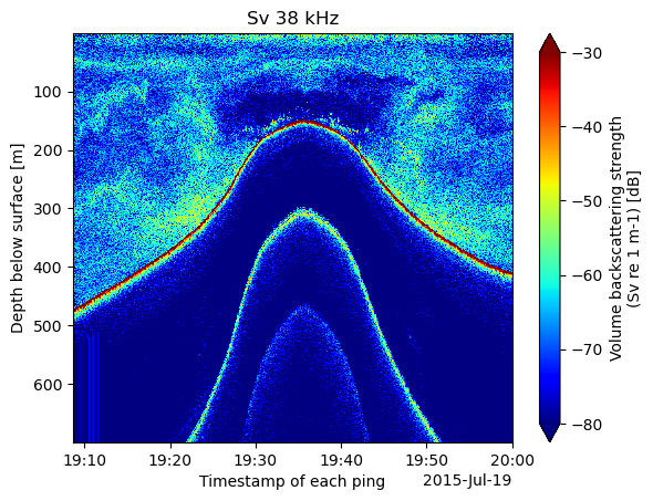
The data in the plot above shows a detected bottom as a ship crosses above a smooth ridge. Beneath the seabed are two harmonics we would like to omit from the plot. We can begin to do that by just plotting data between 0 and 500 meters of depth.

start_depth = 0
end_depth = 500

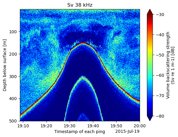
select_depths = (cruise_osdf.depth > start_depth) & (cruise_osdf.depth < end_depth)

Sv_38_subset = Sv_38.where((select_depths), drop=True)

Now when we plot the data it is subsetted to less than 500 meters of depth.

%%time
Sv_38_subset.plot(yincrease=False, cmap='jet', vmin=-80, vmax=-30)
plt.title(f"Sv 38 kHz")

CPU times: user 607 ms, sys: 48.9 ms, total: 656 ms
Wall time: 816 ms

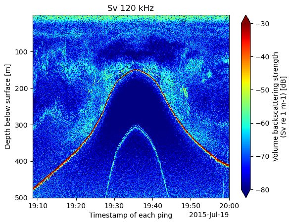
We can also select the corresponding data for 120 and 200 kHz and store them in seperate variables

Sv_18 = cruise_osdf.sel(frequency=18000).where((select_times) & (select_depths), drop=True).Sv
Sv_120 = cruise_osdf.sel(frequency=120000).where((select_times) & (select_depths), drop=True).Sv
Sv_200 = cruise_osdf.sel(frequency=200000).where((select_times) & (select_depths), drop=True).Sv

For comparison, let’s see the 120 kHz echogram with the same depth bounds.

Sv_120_subset = Sv_120.where((select_depths), drop=True)

%%time
Sv_120_subset.plot(yincrease=False, cmap='jet', vmin=-80, vmax=-30)
plt.title(f"Sv 120 kHz")

CPU times: user 587 ms, sys: 68.2 ms, total: 656 ms
Wall time: 775 ms

NDC Workflows

Use the GeoJSON file to get the Area of Interest and query the STAC catalog for items

Old Workflows

Access AWS CESM2 using the AWS open data origin data