Visualization of unstructured grid maps

Contents

Visualization of unstructured grid maps#

[1]:

%load_ext autoreload
%autoreload 2

import os
import numpy as np
os.chdir('/glade/u/home/fengzhu/Github/x4c/docsrc/notebooks')
import x4c
print(x4c.__version__)

2024.8.13

[2]:

dirpath = '/glade/campaign/univ/ubrn0018/fengzhu/CESM_output/timeseries/b.e13.B1850C5.ne30_g16.icesm131_d18O_fixer.Miocene.3xCO2.006'
case = x4c.Timeseries(dirpath, grid_dict={'atm': 'ne30np4', 'ocn': 'g16'})

>>> case.root_dir: /glade/campaign/univ/ubrn0018/fengzhu/CESM_output/timeseries/b.e13.B1850C5.ne30_g16.icesm131_d18O_fixer.Miocene.3xCO2.006
>>> case.path_pattern: comp/proc/tseries/month_1/casename.mdl.h_str.vn.timespan.nc
>>> case.grid_dict: {'atm': 'ne30np4', 'ocn': 'g16', 'lnd': 'ne30np4', 'rof': 'ne30np4', 'ice': 'g16'}
>>> case.vars_info created

CAM-SE#

[3]:

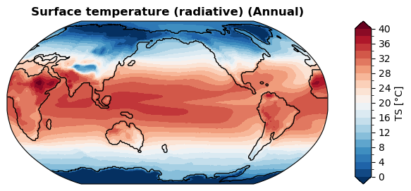
case.load('TS')
da_tas = case.ds['TS'].x['TS'].mean('time')-273.15
da_tas

>>> case.ds["TS"] created

[3]:

<xarray.DataArray 'TS' (ncol: 48602)> Size: 194kB
array([26.467163, 26.114838, 25.527252, ..., 24.563751, 24.704865,
       25.221466], dtype=float32)
Dimensions without coordinates: ncol
Attributes:
    units:         K
    long_name:     Surface temperature (radiative)
    cell_methods:  time: mean
    path:          /glade/campaign/univ/ubrn0018/fengzhu/CESM_output/timeseri...
    gw:            <xarray.DataArray 'gw' (ncol: 48602)> Size: 389kB\narray([...
    lat:           <xarray.DataArray 'lat' (ncol: 48602)> Size: 389kB\n[48602...
    lon:           <xarray.DataArray 'lon' (ncol: 48602)> Size: 389kB\n[48602...
    comp:          atm
    grid:          ne30np4

[4]:

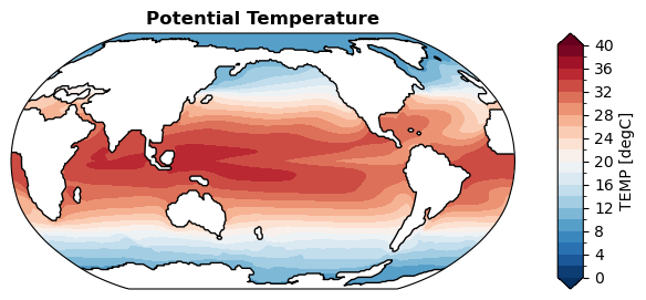
case.load('TEMP')
da_sst = case.ds['TEMP'].x['TEMP'].mean('time').isel(z_t=0)
da_sst

>>> case.ds["TEMP"] created

[5]:

da_sst_rgd = da_sst.x.regrid()
da_sst_rgd

With regridding#

[ ]:

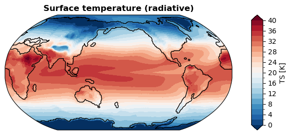
%%time

fig, ax = da_tas.x.regrid().x.plot(
    levels=np.linspace(0, 40, 21),
    cbar_kwargs={
        'ticks': np.linspace(0, 40, 11),
    },
    ssv=da_sst_rgd,   # coastline based on given sea surface variable
)

CPU times: user 1.07 s, sys: 3.85 ms, total: 1.07 s
Wall time: 1.08 s

../_images/notebooks_core-unstructured_grid_maps_8_1.png

[ ]:

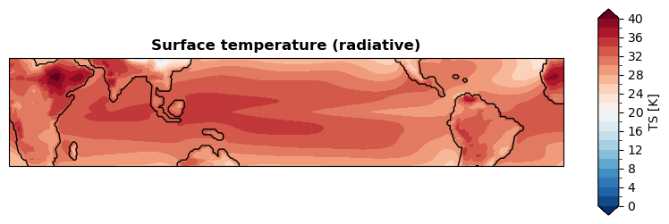
fig, ax = da_tas.x.regrid().x.plot(
    levels=np.linspace(0, 40, 21),
    cbar_kwargs={
        'ticks': np.linspace(0, 40, 11),
    },
    ssv=da_sst_rgd,   # coastline based on given sea surface variable
    latlon_range=(-30, 30, -180, 180),  # plot tripical region
)

../_images/notebooks_core-unstructured_grid_maps_9_0.png

Without regridding#

[ ]:

%%time
fig, ax = da_tas.x.plot(
    levels=np.linspace(0, 40, 21),
    cbar_kwargs={
        'ticks': np.linspace(0, 40, 11),
    },
    ssv=da_sst_rgd,   # coastline based on given sea surface variable
)

CPU times: user 287 ms, sys: 0 ns, total: 287 ms
Wall time: 286 ms

../_images/notebooks_core-unstructured_grid_maps_11_1.png

[ ]:

fig, ax = da_tas.x.plot(
    levels=np.linspace(0, 40, 21),
    cbar_kwargs={
        'ticks': np.linspace(0, 40, 11),
    },
    ssv=da_sst_rgd,   # coastline based on given sea surface variable
    latlon_range=(-30, 30, -180, 180),  # plot tripical region
)

../_images/notebooks_core-unstructured_grid_maps_12_0.png

UXarray vs x4c vs x4c-regrid#

[ ]:

%%time

fig, ax = da_tas.x.plot(
    levels=np.linspace(0, 40, 21),
    cbar_kwargs={
        'ticks': np.linspace(0, 40, 11),
    },
    ssv=da_sst_rgd,   # coastline based on given sea surface variable
    ux=True,          # use UXarray
)

CPU times: user 1.22 s, sys: 11.8 ms, total: 1.23 s
Wall time: 1.17 s

../_images/notebooks_core-unstructured_grid_maps_14_1.png

[ ]:

%%time

fig, ax = da_tas.x.plot(
    levels=np.linspace(0, 40, 21),
    cbar_kwargs={
        'ticks': np.linspace(0, 40, 11),
    },
    ssv=da_sst_rgd,   # coastline based on given sea surface variable
    ux=False,         # don't use UXarray
)

CPU times: user 297 ms, sys: 75 μs, total: 297 ms
Wall time: 296 ms

../_images/notebooks_core-unstructured_grid_maps_15_1.png

[ ]:

%%time

fig, ax = da_tas.x.regrid().x.plot(
    levels=np.linspace(0, 40, 21),
    cbar_kwargs={
        'ticks': np.linspace(0, 40, 11),
    },
    ssv=da_sst_rgd,   # coastline based on given sea surface variable
)

CPU times: user 1.08 s, sys: 116 μs, total: 1.08 s
Wall time: 1.08 s

../_images/notebooks_core-unstructured_grid_maps_16_1.png

POP#

With regridding#

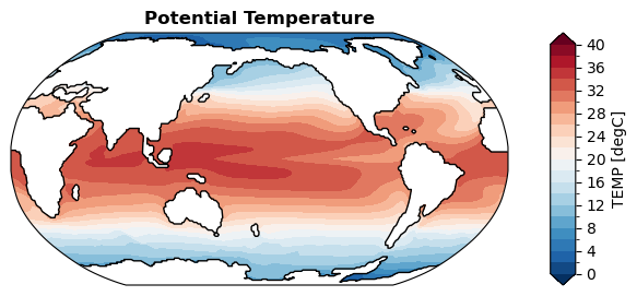
[29]:

%%time

fig, ax = da_sst.x.regrid().x.plot(
    levels=np.linspace(0, 40, 21),
    cbar_kwargs={
        'ticks': np.linspace(0, 40, 11),
    },
)

CPU times: user 2.39 s, sys: 19.8 ms, total: 2.41 s
Wall time: 2.41 s

../_images/notebooks_core-unstructured_grid_maps_19_1.png

Without regridding#

[ ]:

%%time

fig, ax = da_sst.x.plot(
    levels=np.linspace(0, 40, 21),
    cbar_kwargs={
        'ticks': np.linspace(0, 40, 11),
    },
)

CPU times: user 579 ms, sys: 183 μs, total: 579 ms
Wall time: 577 ms

../_images/notebooks_core-unstructured_grid_maps_21_1.png

Case#

Air surface temperature#

[31]:

%%time
# the first time will be slower due to ssv calculation
# ssv will be cached afterwards
fig, ax = case.plot('TS:ann', regrid=True, recalculate_ssv=True)

CPU times: user 4.23 s, sys: 47.8 ms, total: 4.28 s
Wall time: 4.29 s

../_images/notebooks_core-unstructured_grid_maps_24_1.png

[32]:

%%time
fig, ax = case.plot('TS:ann', regrid=True)

CPU times: user 1.08 s, sys: 3.61 ms, total: 1.08 s
Wall time: 1.08 s

../_images/notebooks_core-unstructured_grid_maps_25_1.png

[33]:

%%time
fig, ax = case.plot('TS:ann')

CPU times: user 289 ms, sys: 54 μs, total: 289 ms
Wall time: 288 ms

../_images/notebooks_core-unstructured_grid_maps_26_1.png

[34]:

%%time
fig, ax = case.plot('TS:ann', ux=True)

CPU times: user 1.2 s, sys: 15 ms, total: 1.22 s
Wall time: 1.16 s

../_images/notebooks_core-unstructured_grid_maps_27_1.png

Sea surface temperature#

[ ]:

%%time
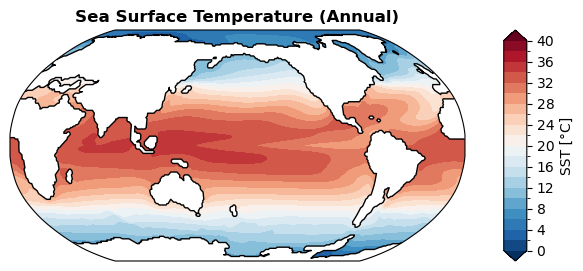
fig, ax = case.plot('SST:ann', regrid=True)  # with regridding

CPU times: user 2.43 s, sys: 20 ms, total: 2.45 s
Wall time: 2.45 s

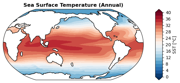
../_images/notebooks_core-unstructured_grid_maps_29_1.png

[59]:

%%time
fig, ax = case.plot('SST:ann')   # without regridding

CPU times: user 593 ms, sys: 82 μs, total: 593 ms
Wall time: 593 ms

../_images/notebooks_core-unstructured_grid_maps_30_1.png