trouble plotting sea ice concentration · python-questions

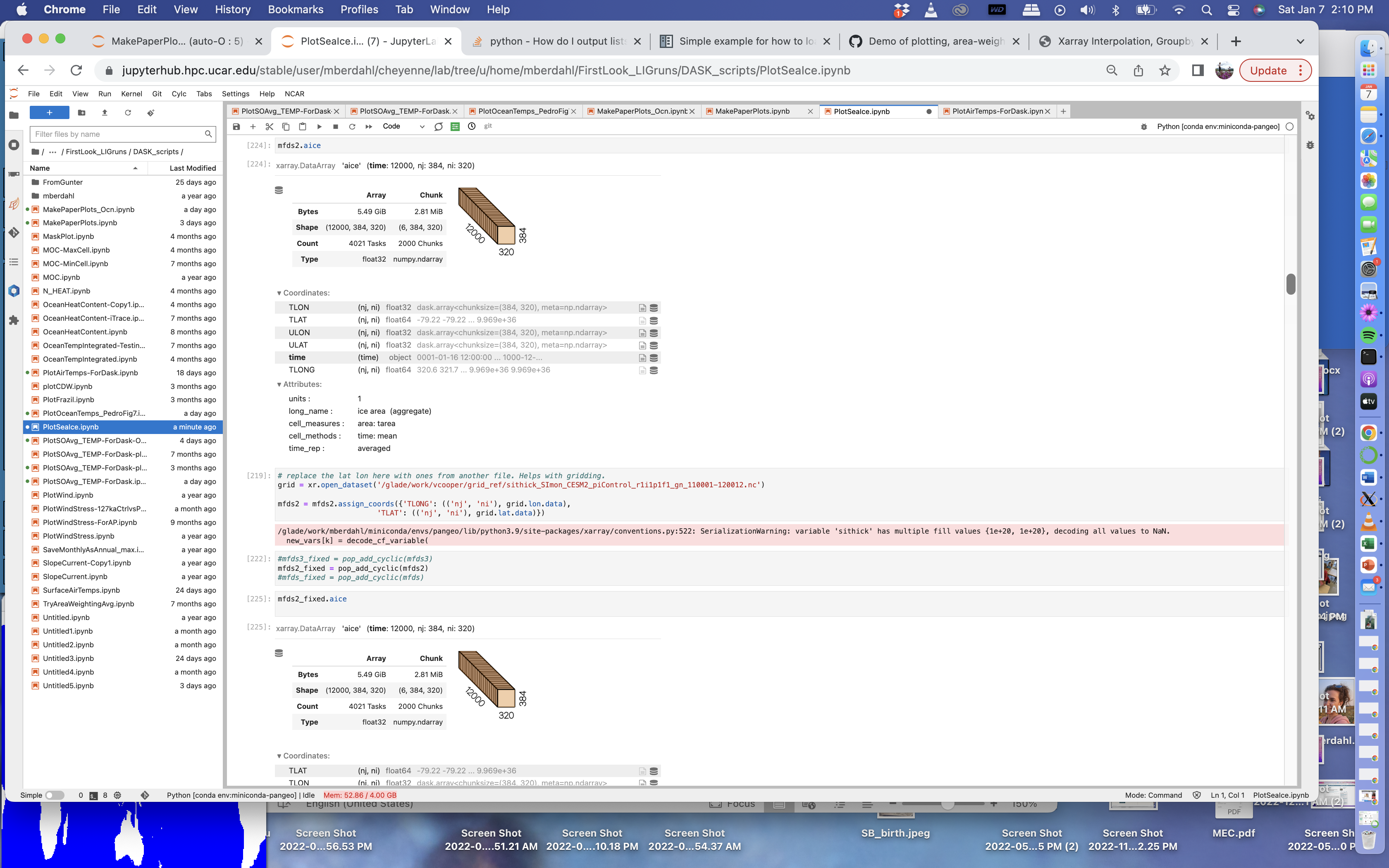
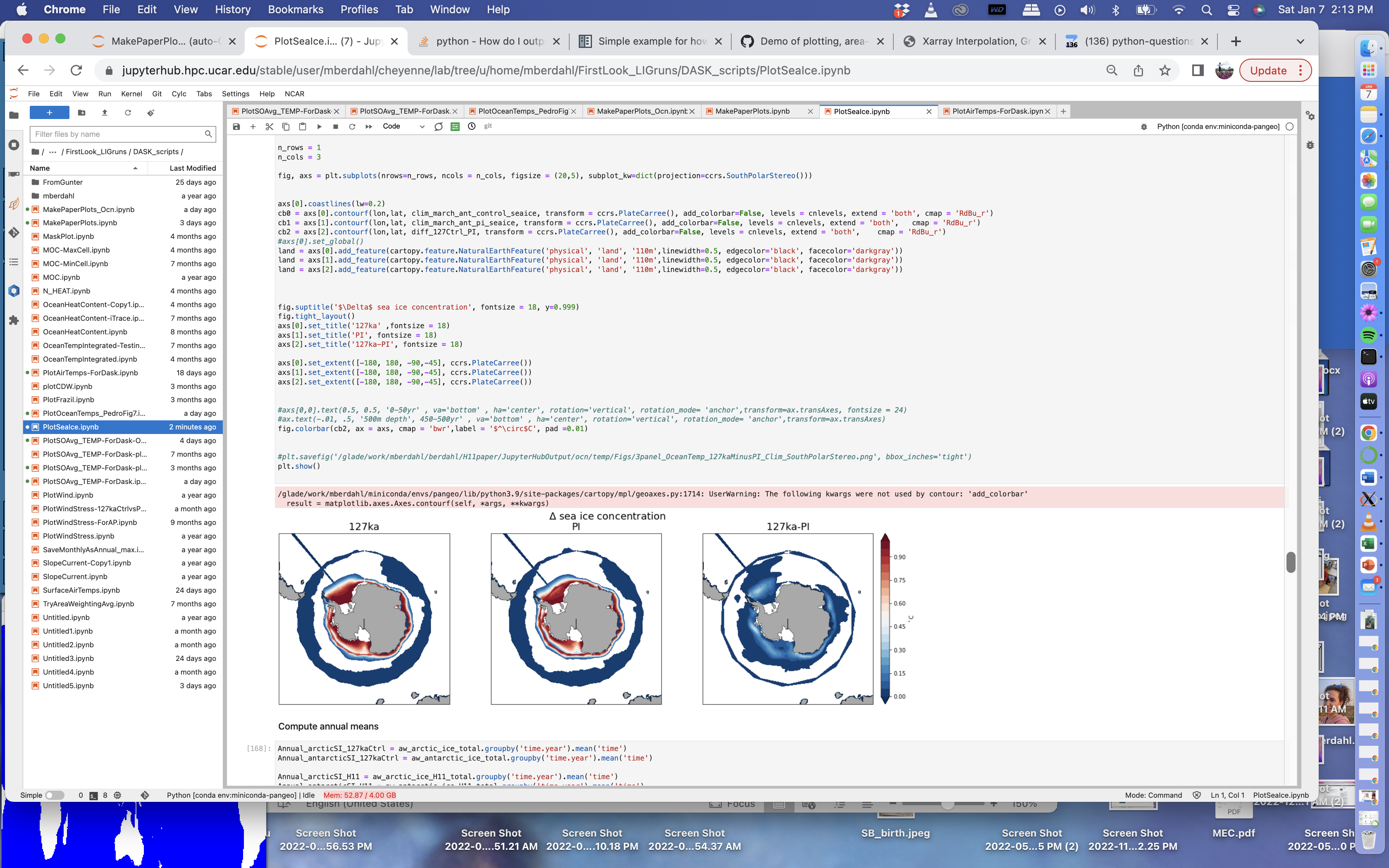
I'm trying to plot a simple sea ice concentration on a projected plot, but I'm getting some erroneous lines in my figures (see attached). My data is CESM2 output. In the past when working with ocean (POP) output, I've had success with replacing the lat/lon grid with that from another file, and then the applying pop_add_cyclic function in order to wrap the lons properly, but this doesn't seem to work with the seaice data. Attached I'm showing a screenshot that displays the details of the original data, then how I replace the lat/lon with a different grid, and then apply the pop_add_cyclic function. After the pop_add_cyclic function is applied, I don't see the dimension ni change, as I would have expected. Can anyone identify what is going wrong here? The pop_add_cyclic function I'm using is:

def pop_add_cyclic(ds):

    nj = ds.TLAT.shape[0]
    ni = ds.TLON.shape[1]

    xL = int(ni/2 - 1)
    xR = int(xL + ni)

    tlon = ds.TLON.data
    tlat = ds.TLAT.data

    tlon = np.where(np.greater_equal(tlon, min(tlon[:,0])), tlon-360., tlon)
    lon  = np.concatenate((tlon, tlon + 360.), 1)
    lon = lon[:, xL:xR]

    if ni == 320:
        lon[367:-3, 0] = lon[367:-3, 0] + 360.
    lon = lon - 360.

    lon = np.hstack((lon, lon[:, 0:1] + 360.))
    if ni == 320:
        lon[367:, -1] = lon[367:, -1] - 360.

    #-- trick cartopy into doing the right thing:
    #   it gets confused when the cyclic coords are identical
    lon[:, 0] = lon[:, 0] - 1e-8

    #-- periodicity
    lat = np.concatenate((tlat, tlat), 1)
    lat = lat[:, xL:xR]
    lat = np.hstack((lat, lat[:,0:1]))

    TLAT = xr.DataArray(lat, dims=('nlat', 'nlon'))
    TLON = xr.DataArray(lon, dims=('nlat', 'nlon'))

    dso = xr.Dataset(coords={'TLAT': TLAT, 'TLON': TLON})

    # copy vars
    varlist = [v for v in ds.data_vars if v not in ['TLAT', 'TLON']]
    for v in varlist:
        v_dims = ds[v].dims
        if not ('nlat' in v_dims and 'nlon' in v_dims):
            dso[v] = ds[v]
        else:
            # determine and sort other dimensions
            other_dims = set(v_dims) - {'nlat', 'nlon'}
            other_dims = tuple([d for d in v_dims if d in other_dims])
            lon_dim = ds[v].dims.index('nlon')
            field = ds[v].data
            field = np.concatenate((field, field), lon_dim)
            field = field[..., :, xL:xR]
            field = np.concatenate((field, field[..., :, 0:1]), lon_dim)
            print(field.shape)
            dso[v] = xr.DataArray(field, dims=other_dims+('nlat', 'nlon'),
                                  attrs=ds[v].attrs)


    # copy coords
    for v, da in ds.coords.items():
        if not ('nlat' in da.dims and 'nlon' in da.dims):
            dso = dso.assign_coords(**{v: da})


    return dso

Mira Berdahl (Jan 09 2023 at 19:58):

I think I've figure this out -- in the sea ice file, the lat/lon contained masked values in locations with land. After using the grid from pop_tools instead of the lat/lon associated with the sea ice data, it works:

# using pop tools, get the region mask.
grid_name = 'POP_gx1v7'  # our 1 degree pop grid.
grid = pop_tools.get_grid(grid_name)

import cmocean as cm
import cartopy.feature as cfeature

f, ax = plt.subplots(subplot_kw=dict(projection=ccrs.SouthPolarStereo()))

p = ax.pcolormesh(grid.TLONG,
              grid.TLAT,
              mfds3_onetime.aice,
              transform=ccrs.PlateCarree(),
              vmin=0, vmax=1, cmap=cm.cm.ice)

f.colorbar(p, label='sea ice concentration [%]')
ax.set_title('JJA Sea Ice Concentration (1970-2000)')

ax.set_extent([-180, 180, -90,-45], ccrs.PlateCarree())
# Add land.
ax.add_feature(cfeature.LAND, color='#a9a9a9', zorder=4)

Stream: python-questions

Topic: trouble plotting sea ice concentration

Mira Berdahl (Jan 07 2023 at 22:18):

Mira Berdahl (Jan 09 2023 at 19:58):