Stephen Yeager (Sep 23 2020 at 22:36): Stephen Yeager (Sep 23 2020 at 22:36):
Venue for ongoing discussion of how to improve FOSI sea ice simulation
Fred Castruccio (Sep 23 2020 at 23:15):I have a question regarding the albedo.
We are using dt_mlt = 0.5. It was 1 in LENS.
And r_snw is 1.6. It was 1.75 in LENS.
Are the changes associated with the change from CICE4 to CICE5?
If I am not mistaken, I think the LENS parameters will increase the albedo and result in larger sea ice volume/extent.
If yes, why are we more conservative with those parameters in CESM2 than in LENS?
Who Kim (Sep 23 2020 at 23:16):What we had on the table were:
1) albedo change + T&S restoring to modeled salinity-dependent Tfrz and observed S under sea ice
2) albedo change + LWDN reduction (by 5 W m^-2 north of 60N)
with a possible modification of air temperature and/or further tuning of albedo.
(1) and (2) show very similar Arctic sea-ice volume and extent. But, it looks to me (1) is slightly better than (2) in the Souther Ocean. @Marika Holland suggested that (2) would be a safer option because of summer melting, which increases in time, that could decrease Tfrz, thus can compensate the sea ice decline in the later years. However, in this simulation, S is also restored to observed climatology, so I think we can avoid Tfrz messed up (Could @Marika Holland chime in to confirm if my interpretation is right?). We can also restore T to max(Tfrz,Trst), but the caveat is that it is less effective than restoring just to Tfrz. Assuming my interpretation is right, I think (1) or (1) with some further tuning is the most viable option because it has the edge in the Souther Ocean...
Fred Castruccio (Sep 23 2020 at 23:25):I like Bill Large suggestion during the section meeting this morning to look at the albedo used by JRA to come up with the LWDN forcing.
Stephen Yeager (Sep 23 2020 at 23:28):@Who Kim Why do we need to restore to SSS under ice in (1)? Your new sensitivities show that it doesn't do much, the SST restoring to Tfrz(S) is what is important. If we eliminate SSS restoring, then I think Marika's worry is eliminated because enhanced summer melting will increase Tfrz, but the model will be restored to that new higher Tfrz (with a weighting by ice fraction).
Marika Holland (Sep 23 2020 at 23:53):My concern with the restoring to Tfrz under ice is that as the ice thins and reduces in concentration, the under-ice temperature should in reality become elevated above Tfrz because of absorbed SW. This then impacts the amount of summer melting and the resulting September ice concentration. If we restore to Tfrz throughout the simulations, then the restoring flux will be larger later in the record when thin/low concentration ice is present and this can affect the time evolution of the simulation in non-physical ways. Because of this, I think that adjustments to the forcing (the LW down and/or air temperature) may be "safer".
Marika Holland (Sep 24 2020 at 00:14):@Fred Castruccio Regarding the question about the albedo values, dt_mlt=0.5 will give a higher albedo than dt_mlt=1 (as in LENS). The dt_mlt defines the temperature below freezing at which the snow transitions to wet snow values (with lower albedos). The R_snw=1.6 is actually equivalent to R_snw=1.75 (as in LENS) because we have a minimum snow grain radius value and the model reaches that for an R_snw value of 1.6. So the albedos in Who's runs are actually higher than the LENS values for snow covered ice.
Fred Castruccio (Sep 24 2020 at 00:46):@Marika Holland Thanks for the clarification. So dt_mlt is not a delta in temperature but an absolute value? LENS transition to wet snow occurs at -1C while CESM2 transition occurs -0.5C. Is that right?
Fred Castruccio (Sep 24 2020 at 01:10):@Marika Holland The restoring is weighted by the ice fraction. So when the ice start to melt the strength of the restoring will be greatly reduced. An option to make it even safer is to restore to the max between TFRZ and an observational SST product. If we do that, we may want to upgrade to a more recent product than PHC2, like PHC3, or maybe EN4.
Marika Holland (Sep 24 2020 at 03:27):@Fred Castruccio correct - the dt_mlt value is basically an absolute value and so dt_mlt=0.5 means the transition to a melting snow grain radius starts at Tsfc= -0.5C
Marika Holland (Sep 24 2020 at 03:38):It's good to know that the restoring is weighted by the ice fraction, that should help. However, I still am uncomfortable with adding a flux that varies over time and can compensate for a real feedback in the system. Given that the ice-ocean heat exchange depends on the salinity dependent freezing temperature (since that will be the temperature of the ice base), I think it can be problematic to use an observed SST product that is referenced to a different freezing temperature. It may make more sense to use the difference from freezing somehow in the restoring.
Who Kim (Sep 24 2020 at 04:23):@Marika Holland Thanks for the clarification. @Stephen Yeager My interpretation might be wrong, but I think S restoring might be needed because SSS can be fresher (than obs) during summer without restoring under warming because there could be a positive feeback between salinity and Tfrz: that is, weaker sea-ice decline than observed during winter due to strong constrained by Tfrz > freshwater increase during summer due to ice melt > increasing Tfrz > stronger constained by Tfrz during winter.
Stephen Yeager (Sep 24 2020 at 14:41):After all this back and forth, I'm confused about next steps for zeroing in on FOSI mods to hand over to the BGC group. Do we need a zoom call? My takeaway is that Dave/Marika would like to see another sensitivity combining: enhanced albedo mods + LWDN reduction (both hemispheres) + Tair mods (NH only?). Is that correct?
Fred Castruccio (Sep 24 2020 at 16:18):I think a zoom call may be the most efficient way to move forward.
Fred Castruccio (Sep 24 2020 at 16:32):@Marika Holland I agree that the main complication is that observed SST product don't use a salinity dependent freezing temperature. The model tends to have a higher freezing point (-1.5C or -1.6C) than PHC2 (-1.8C). Using the max between Tfrz and Trst is a simple attend at mitigating the issue. Using the difference from freezing is ultimately a better approach I think but can we get an observed freezing point we can rely on?
David Bailey (Sep 24 2020 at 17:15):Marika and I chatted and we could do additional albedo mods (dt_mlt = 0.2, rsnw_mlt = 800). However, we are both concerned about the Antarctic and we would like to extend the LW changes there as well as potentially temperature changes. As Marika said, she is concerned about the variability in the sea ice with the restoring. So, it would be good to assess the 2010 state in the runs. This is also the initial state we need for the prediction runs right? In terms of the default configuration for G compsets moving forward, we need to do more of a detailed assessment and that should be a longer term goal. We are fine with the albedo changes, but it would be good to assess the forcing changes against observations and also assess variability with the restoring. We are happy to chat on a Zoom call tomorrow if needed.
Marika Holland (Sep 24 2020 at 17:49):As Dave mentions, I'd be available for a zoom call tomorrow. Perhaps 9am?
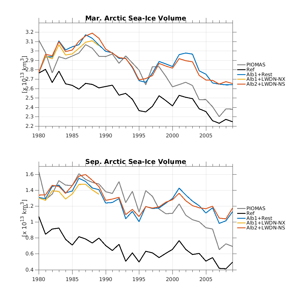
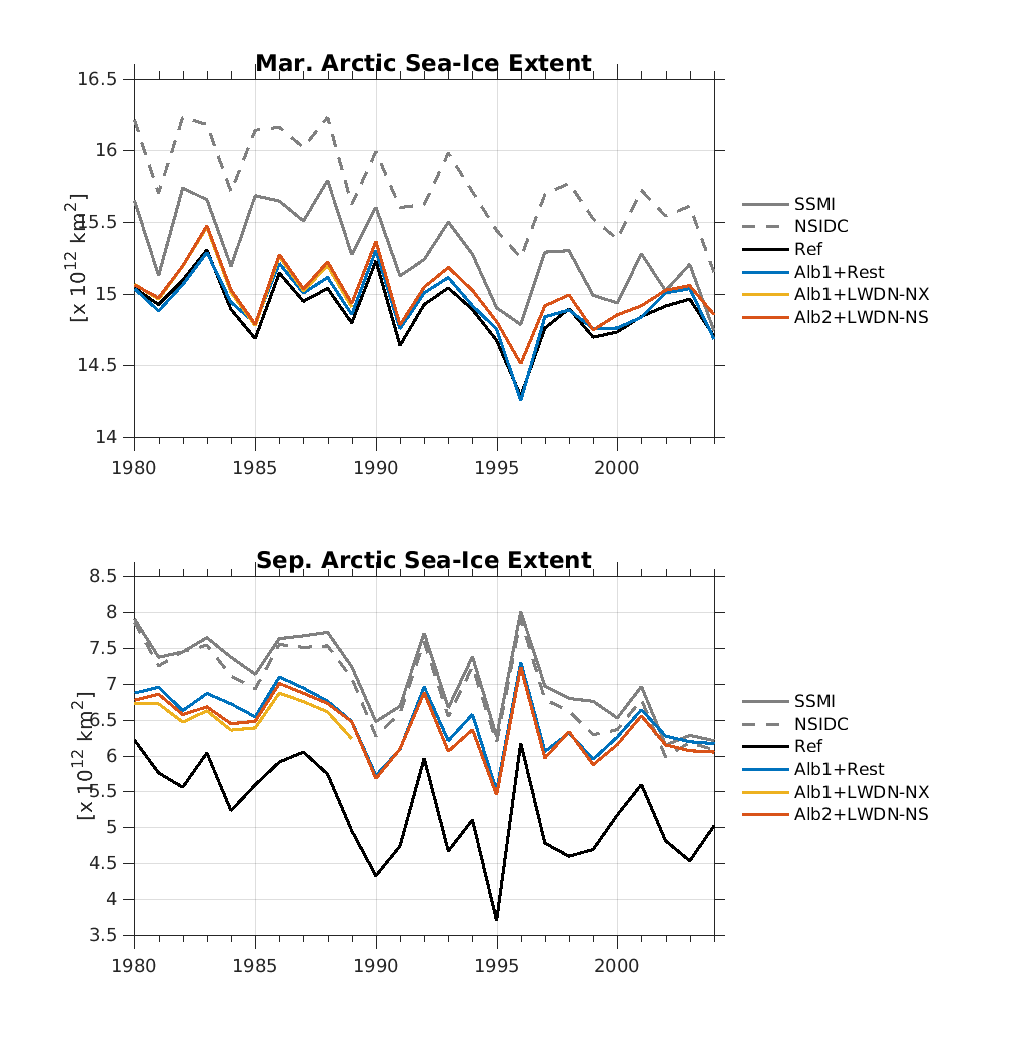
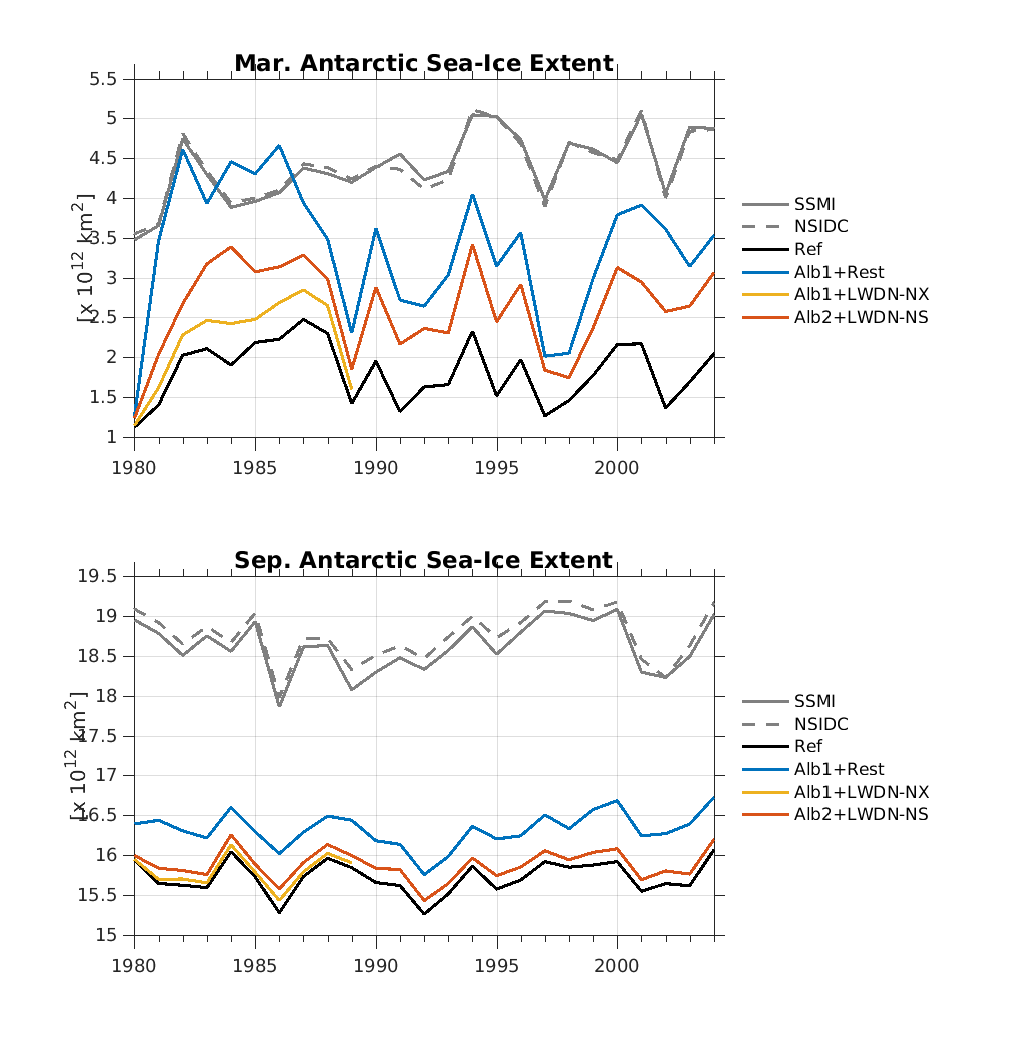
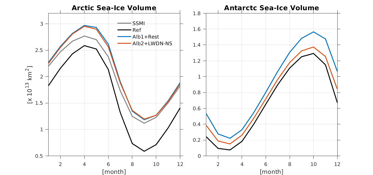
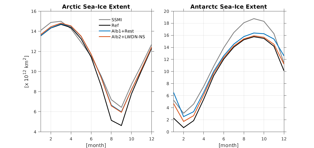
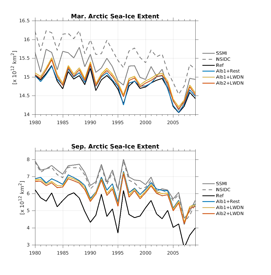
Who Kim (Sep 28 2020 at 17:09):I have run a new case (modified albedo + LWDN reduction in both hemispheres) through 2009 (from 1980). I have also extended albedo+restoring through 2009. The attached plots below are some diagnositics from these experiments (label Alb2+LWDN-NS and Alb1+Rest, respectively). For the monthly climatology, the last 20 year mean (1990-2009) is plotted. In time series plots, the first 10 years of the (original) albedo + NH LWDN reduction experiment (Alb1+LWDN-NX) are also plotted as a reference for Alb2+LWDN-NS. in the extent time series, I have also included the extent computed from SSMI remapped onto gx1 (interestingly the extent is significantly different from NSIDC only in March and in the Arctic).
In the Arctic, Alb2+LWDN-NS appears to perform overall similar to Alb1+Rest, but better in terms of change (decline). In the Souther Ocean, Alb2+LWDN-NS appears to be still worse than Alb1+Rest in terms of ice extent, but the too strong March extent interannual variability in Alb1+Rest is somewhat suppressed.
ice_vol_NH_Mar_Sep_ts_select.png
ice_ext_NH_Mar_Sep_ts_select.png
ice_ext_SH_Mar_Sep_ts_select.png
ice_vol_mon_clim.png
ice_ext_mon_clim.png
David Bailey (Sep 29 2020 at 20:06):I have run the sea ice diagnostics for this run. Still not quite enough in the SH.
Stephen Yeager (Sep 29 2020 at 21:20):What are your thoughts on the discrepancy with PIOMAS trends in recent years in the new runs? We are going to try a couple other runs before meeting again to discuss.
Fred Castruccio (Sep 29 2020 at 22:17):@Marika Holland @Laura Landrum I remember helping you setting up a simulation with interior restoring a few years ago in order to investigate Antarctic sea ice trend and try to better understand the mismatch between the observed trend and the trend simulated by CESM. Can you refresh my memory regarding the details of that experiment? Also do you remember if the restoring had a positive impact on the sea bias? Thanks!
Marika Holland (Sep 29 2020 at 22:23):@Fred Castruccio We talked about these interior nudging runs but never actually performed them.
Marika Holland (Sep 29 2020 at 22:40):@Stephen Yeager @Who Kim I'm not certain about the discrepancy with the PIOMAS timeseries. Who's runs do seem to have low ice thinning in the Arctic. The PIOMAS data is quite uncertain though. They assimilate ice concentration but no thickness.
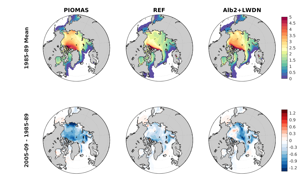
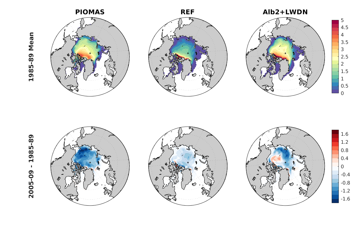
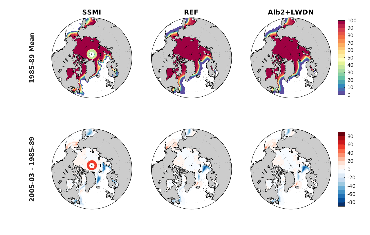
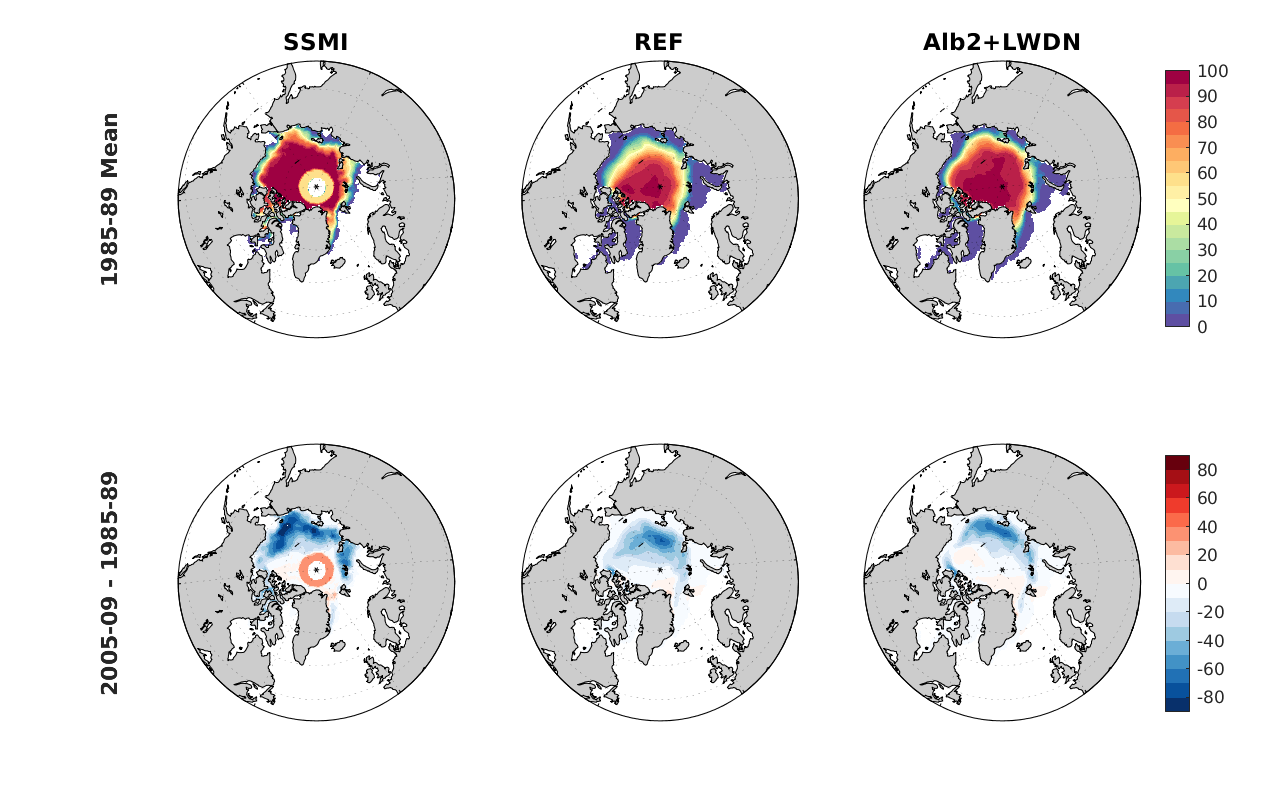
Who Kim (Sep 30 2020 at 05:14):I made spatial difference plots between 2005-2009 and 1985-1989 for March and September. In these plots, I am only showing Alb2+LWDN-NS along with observations and REF, but similar differences are found for Alb1+Rest.
In addition to the difference in the overall amplitude of the thickness decline, the thickness difference plots show a quite different pattern between PIOMAS and FOSIs: FOSIs shows a weaker decline or even an increase around the Beaufort gyre in both seasons, which appears to be the reason for the weaker thickness decline in FOSIs compared to PIOMAS. This seems to be related to a strengthening of the Beaufort gyre in the later period, so that sea ice is converging there in FOSIs. There is no such a sign of a reduced decline near the Beaufort gyre in PIOMAS.
Unlike thickness, the observed (SSMI) ice concentration difference is reasonably reproduced in FOSIs, except that the September decline takes place near the poleward biased sea-ice edge in FOSIs.
hi_Mar_diff_NH.png
hi_Sep_diff_NH.png
aice_Mar_diff_NH.png
aice_Sep_diff_NH.png
Gokhan Danabasoglu (Sep 30 2020 at 18:51):Well, the plot thickens, figuratively. If the PIOMAS assimilation does not use "proper" winds, then perhaps increase in volume around 2000 may have a chance of being realistic.
David Bailey (Oct 01 2020 at 20:22):There is a nice paper from Zack Labe that compares PIOMAS to some observational products. Basically, there is a thin bias in the PIOMAS. Who, do you have the extent plots up to 2009? It looks like yours stop at 2005. jcli-d-17-0436.1.pdf
Marika Holland (Oct 01 2020 at 22:56):I believe that PIOMAS is driven with NCEP forcing. It does assimilate ice concentration though which will modify the ice thickness.
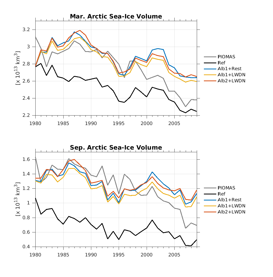
Who Kim (Oct 02 2020 at 17:07):@David Bailey , Attached is the Arctic sea ice volume time series up to 2009.
@Stephen Yeager , @Fred Castruccio , @Gokhan Danabasoglu , The yellow line in this plot is the experiment with the original albedo change extended to 2009 (Alb1+LWDN) that we discussed early this week. No noticeable difference compared to the red line (Alb2+LWDN)
ice_vol_NH_Mar_Sep_ts_select.png
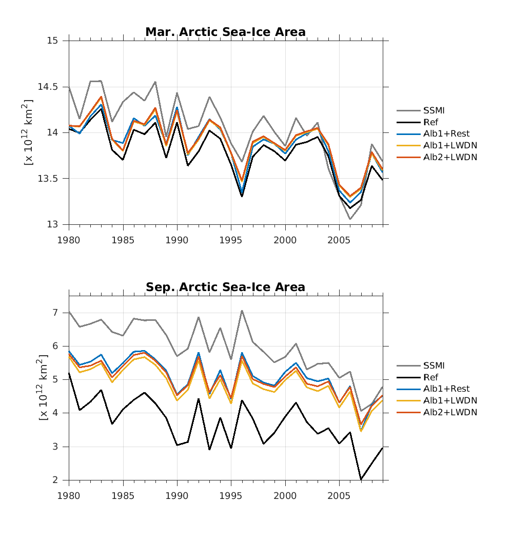
David Bailey (Oct 02 2020 at 17:16):What about ice area and extent timeseries through 2009?
Who Kim (Oct 02 2020 at 22:36):Ice Area
ice_area_NH_Mar_Sep_ts_select.png
Ice extent
ice_ext_NH_Mar_Sep_ts_select.png
David Bailey (Oct 05 2020 at 15:49):These look good. These for the SH as well will be good. I think the volume discrepancy after 2000 with the PIOMAS is related to the forcing (JRA versus NCAR-NCEP). Notice that the trends in the original FOSI run are not as strong as PIOMAS.
Keith Lindsay (Oct 05 2020 at 16:31):I just noticed that the sensitivity runs for generating ocean/ice initial state are using kappa_isop_deep=0.2. My recollection was that we were going to go with kappa_isop_deep=0.1, like we did in Kristen's runs.
I'm concerned that the Southern Ocean sea ice solution, particularly its sensitivity to the various configurations being evaluated, may depend on this parameter in unknown ways.
Matt Long (Oct 05 2020 at 17:07):cc @Who Kim
Stephen Yeager (Oct 05 2020 at 17:22):Since Who stepped up to perform these sensitivity runs, we decided to use his old JRA55-do case (using 0.2) as the control just to make things easy. We can switch over to the new kappa_isop_deep moving forward.
Who Kim (Oct 05 2020 at 17:27):Because we aimed initially a short integration, I didn't care much about kappa difference. But, I speculate that sea ice could be thicker with 'kappa_isop_deep=0.1' because excessive bottom water formation is reduced (thus, the upper ocean is likely colder).
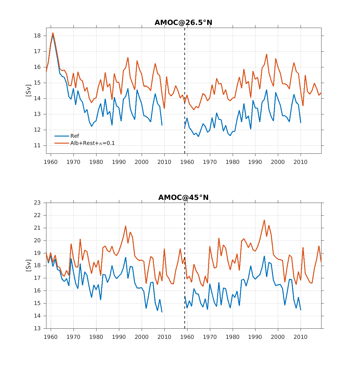
Who Kim (Oct 21 2020 at 22:00):@Keith Lindsay , The case directory of the latest experiment (Alb+Rest+kappa=0.1) is /glade/work/whokim/cesm/cesm2_g/g210.GIAF_JRA.v14.gx1v7.SMYLE.ice_IC.001
Who Kim (Oct 22 2020 at 15:08):AMOC in this experiment is about 2 Sv stronger the the reference case. So, the reduced winter sea ice concentration around the ice edge might be related to stronger heat transport. I suspect that the restoring under sea ice is responsible for this AMOC increase. In the reference case, the entire Arctic Ocean and Nordic Seas have a fresh bias. The reduced bias with the restoring might enhances deep water formation.
Stephen Yeager (Oct 22 2020 at 15:22):Variability looks the same, and mean@26.5N is a better match to RAPID, so I'm thinking this is OK
Gokhan Danabasoglu (Oct 22 2020 at 18:36):I thought a bit more about yesterday's discussion on how we proceed with the fully-coupled simulations. We have 3 sets of albedo settings for the sea-ice model. The default used in our CMIP6 CESM2 simulations; tuned albedos used in CESM2(CAM6) simulations; and the ones used for our CESM2(FOSI) case. As discussed, we will perform some sensitivity simulations for the actual prediction simulations. However, if we decide to go with the second, i.e., the tuned albedos, for these CESM2(CAM6) simulations, if we ever perform prediction simulations with the high-top model version to evaluate prediction sensitivity to model top, that is, CESM2(WACCM6), what albedos will we use? My worry is that we are opening the door to changes potentially in other component models as well with the thinking that we are after the "best possible solutions" in each configuration. This takes me back to the discussions that we had in late 1990s and early 2000s as to what we should do.
Last updated: May 16 2025 at 17:14 UTC