Matt Long (Sep 22 2020 at 12:56): Matt Long (Sep 22 2020 at 12:56):
@Colleen Petrik, what is the status of the FEISTY code? Do you have it in a GitHub repo? It would be great to start to poke around the code and consider how best to facilitate offline applications—and begin moving toward the online model.
Colleen Petrik (Sep 22 2020 at 16:57):@Matt Long , I do have it on GitHub, but it is a bit of a mess. I'm too much of a git novice to utilize branches, so I keep different version in separate folders instead. The code also needs to be streamlined. Maybe the best place for you to start is this one: https://github.com/cpetrik/FEISTY/tree/master/CODE/clim_complete
Matt Long (Sep 22 2020 at 17:34):Awesome, thanks! Can we schedule a walk thru in a couple of weeks? I would like to invite @Kristen Krumhardt, @Michael Levy and possibly @Zephyr Sylvester (if she has time).
I think the key thing is to identify a refactoring plan. We might want to consider a code base capable of supporting both offline and online applications.
In the context of this effort, it will be really useful to have a reference solution against which to check answers.
Colleen Petrik (Sep 24 2020 at 00:40):@stream I can give a walk through in Oct.
Matt Long (Jun 02 2021 at 15:42):@Colleen Petrik, I was starting to poke around the FEISTY code you have linked above. Do you have an example of the code being called? I would like to develop a better understanding of the calling tree.
Colleen Petrik (Jun 02 2021 at 18:47):@Matt Long , the code calling tree looks like Make.m -> Simulation -> sub_futbio.m
Make just picks the simulation. The example simulation in that repository is the ESM2.6-COBALT Climatology. The simulation code has some set-up for loading the gridfile and the forcing file(s) and creating the netcdf files for saving in addition to calling the main program "sub_futbio." The main program is where the majority of the subroutines get called. e.g. metabolism, encounter, ingestion, consumption, reproduction, etc. Let me know if you want anything more specific than that.
Colleen Petrik (Oct 07 2021 at 23:23):@Matt Long and @Michael Levy , I have pushed all FEISTY documentation, including a check table of input and output values, to my github repo.
https://github.com/cpetrik/fish-offline/tree/main/docs
Matt Long (Oct 08 2021 at 12:28):thanks @Colleen Petrik!
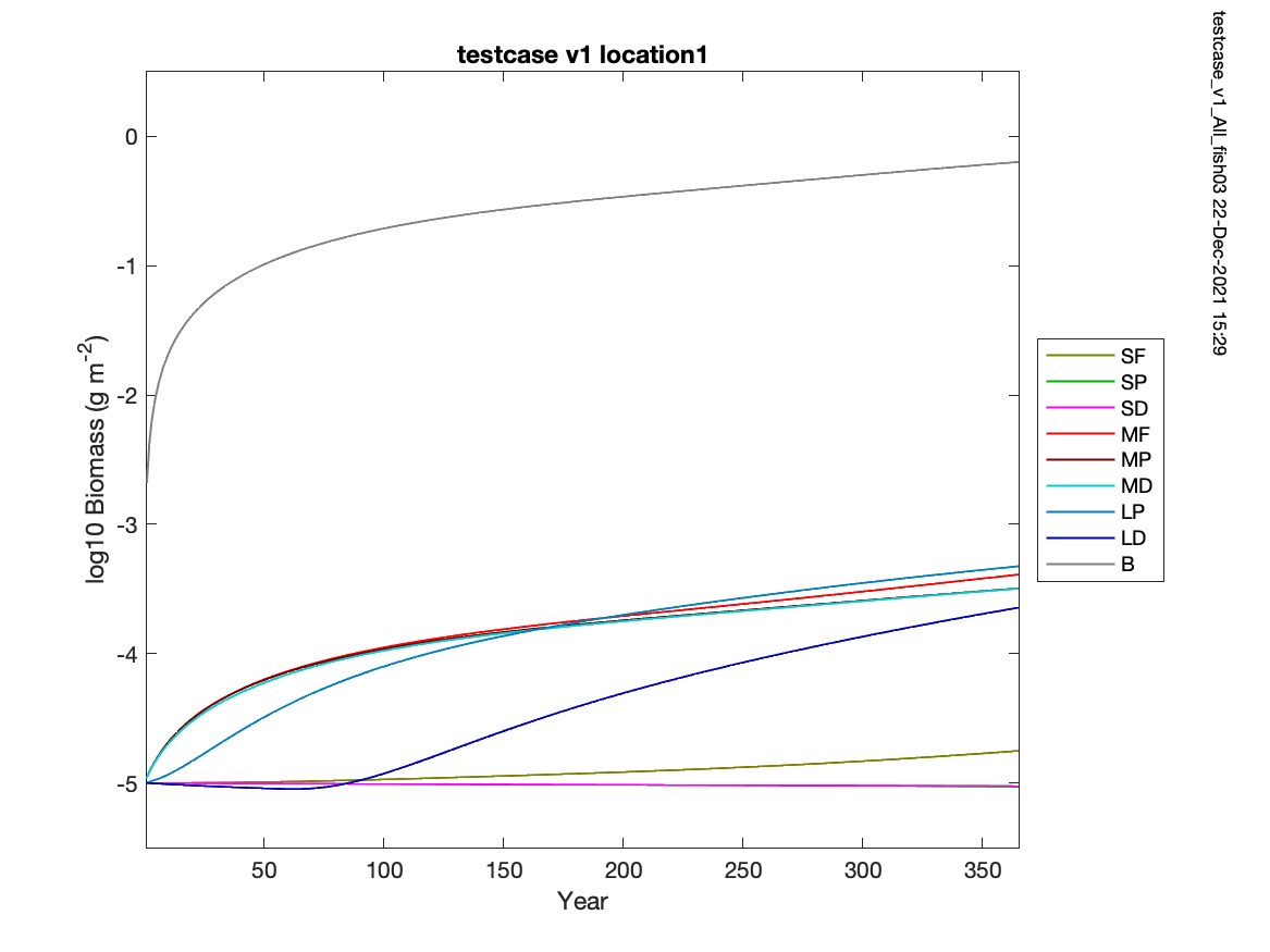
Colleen Petrik (Dec 22 2021 at 23:38):@Matt Long , @Michael Levy , @Zephyr Sylvester : I did a quick run of the testcase using my Matlab code and the testcase default parameters, bathymetry, and cyclical forcing. It results in an increase in biomass of all types, not a decrease. Definitely something to dig into in the new year. testcase_v1_All_fish03_ts_logmean_biomass_location1.png
Michael Levy (Jan 05 2022 at 20:47):@Colleen Petrik can you point me to the matlab code you ran? I'm going to do some side-by-side comparisons of the matlab and python code bases, and maybe also try to do some single-time-step runs with the matlab code on cheyenne to see if I can pinpoint where the issue(s) in the python code is (are)
Colleen Petrik (Jan 06 2022 at 00:20):@Michael Levy , they are in my FEISTY git repo: https://github.com/cpetrik/fish-offline/tree/main/MatFEISTY . The main file is ``testcase.m''. Let me know if you need any help navigating the subroutines.
Colleen Petrik (Jan 06 2022 at 23:27):Hi @Michael Levy . Today I looked through default_settings.yml and process.py for issues. I could not find anything in process.py, but there were a number of default settings that were wrong. I modified them, one at a time, to the correct values, but they did not have any effect and the biomasses of all groups followed the same trajectory as before. For my next course of action, I will look at the outputs of each subroutine/function after one time step in the Matlab and Python versions. I have attached the updated default settings for you to work with. default_settings_CPedits.yml
Michael Levy (Jan 07 2022 at 20:47):@Colleen Petrik thanks for that updated settings file -- I'm currently adding a bunch of disp() calls to your matlab driver and making sure I am getting similar values in the python code. The encounter code looks okay, and I found a bug in the consumption code:
diff --git a/feisty/core/process.py b/feisty/core/process.py
index 9906882..a7bc0d0 100644
--- a/feisty/core/process.py
+++ b/feisty/core/process.py
@@ -202,7 +202,7 @@ def compute_consumption(
     """

     for i, link in enumerate(food_web):
-        enc = consumption_rate_link[i, :]
+        enc = encounter_rate_link[i, :]
         cmax = consumption_rate_max_pred[link.i_fish, :]
         enc_total = encounter_rate_total[link.i_fish, :]
         consumption_rate_link[i, :] = cmax * enc / (cmax + enc_total)
With that fix in place, consumption numbers look better but biomass is still decreasing (looking at group in ["Mf", "Mp", "Md", "Lp", "Ld"])
Michael Levy (Jan 08 2022 at 00:26):@Matt Long more issues with the encounter rate... In the matlab code, we only subtract the .td value from 1 when computing the Md.enc_be (Md_benthic_prey), Lp.enc_d (Lp_Md), Ld.enc_d (Ld_Md), and Ld.enc_be (Ld_benthic_prey) encounters. So I think the if link.prey.is_demersal logic isn't quite what we want, but I'm not sure what to replace it with. Currently I'm seeing an encounter rate of 0 in the python code for both 'Mf_Sd' and 'Mp_Sd', and I think it's tied to the fact that Sd is demersal but t_frac_pelagic_static=1. This might not be right because changing t_frac_pelagic_static affects the encounter rate for Sd_Zoo, without changing it for the two medium-size classes preying on Sd... so I'm a little confused.
Matt Long (Jan 08 2022 at 01:02):I’ll need to look at this in detail
Matt Long (Jan 08 2022 at 13:22):Michael Levy said:
Colleen Petrik thanks for that updated settings file -- I'm currently adding a bunch of
disp()calls to your matlab driver and making sure I am getting similar values in the python code. The encounter code looks okay, and I found a bug in the consumption code:diff --git a/feisty/core/process.py b/feisty/core/process.py index 9906882..a7bc0d0 100644 --- a/feisty/core/process.py +++ b/feisty/core/process.py @@ -202,7 +202,7 @@ def compute_consumption( """ for i, link in enumerate(food_web): - enc = consumption_rate_link[i, :] + enc = encounter_rate_link[i, :] cmax = consumption_rate_max_pred[link.i_fish, :] enc_total = encounter_rate_total[link.i_fish, :] consumption_rate_link[i, :] = cmax * enc / (cmax + enc_total)With that fix in place, consumption numbers look better but biomass is still decreasing (looking at
group in ["Mf", "Mp", "Md", "Lp", "Ld"])
Excellent work!
Matt Long (Jan 08 2022 at 13:30):In the Matlab code, sub_init_fish_spin.m,
Sd.td = ones(NX,1);
So I think t_frac_pelagic_static = 1 for Sd is correct. These are larval demersal fish.
Matt Long (Jan 08 2022 at 14:03):Regarding the logic on if link.prey.is_demersal, I think the logic I had is correct. Here's why I think so.
I introduced a variable t_frac_prey_pred which is the fraction of time the predator spends in the region with it's prey. This corresponds to tprey in the sub_enc Matlab function API.
The variable t_frac_pelagic_pred is always the fraction of time the predator spends in the pelagic zone. I think this implies that regardless of the predator type (i.e., whether is_demersal is true or false), the logic should be
            if link.prey.is_demersal:
                t_frac_prey_pred = 1.0 - t_frac_pelagic_pred
The demersal groups are
MdLdbenthic_preyThe settings are consistent with this.
Here's what the matlab code has:
Sf.enc_zm:  prey: Zoo, tprey = Sf.td
Sp.enc_zm:  prey: Zoo, tprey = Sp.td
Sd.enc_zm:  prey: Zoo, tprey = Sd.td

Mf.enc_zm:  prey: Zoo, tprey = Mf.td
Mf.enc_f:  prey: Sf, tprey = Mf.td
Mf.enc_p:  prey: Sp, tprey = Mf.td
Mf.enc_d:  prey: Sd, tprey = Mf.td

Mp.enc_zm:  prey: zoo, tprey = Mp.td
Mp.enc_f:  prey: Sf, tprey =  Mp.td
Mp.enc_p:  prey: Sp, tprey =  Mp.td
Mp.enc_d:  prey: Sd, tprey =  Mp.td

Md.enc_be:  prey: benthic, tprey = 1-Md.td

Lp.enc_f:  prey: Mf, tprey = Lp.td
Lp.enc_p:  prey: Mp, tprey = Lp.td
Lp.enc_d:  prey: Md, tprey = 1-Lp.td

Ld.enc_f:  prey: Mf, tprey = Ld.td
Ld.enc_p:  prey: Mp, tprey = Ld.td
Ld.enc_d:  prey: Md, tprey = 1-Ld.td
Ld.enc_be: prey: benthic, tprey = 1-Ld.td
I think you can confirm that the is_demersal dependence is correct.
On this last point:
Currently I'm seeing an encounter rate of 0 in the python code for both 'Mf_Sd' and 'Mp_Sd', and I think it's tied to the fact that Sd is demersal but t_frac_pelagic_static=1. This might not be right because changing t_frac_pelagic_static affects the encounter rate for Sd_Zoo, without changing it for the two medium-size classes preying on Sd... so I'm a little confused.
This does seem strange, that the t_frac_pelagic_static of prey doesn't affect the encounter rate.
Michael Levy (Jan 08 2022 at 17:20):Matt Long said:
The demersal groups are
MdLdbenthic_prey
Shouldn't Sd be in that group as well?
    - name: Sd
      size_class: small
      functional_type: demersal
I guess I'm confused about why tprey = Mf.td and Mp.td instead of 1 - Mf.td and 1 - Mp.td in the lines
Mf.enc_d:  prey: Sd, tprey = Mf.td
Mp.enc_d:  prey: Sd, tprey =  Mp.td
That does not seem consistent with the link.prey.is_demersal logic in the python code (but perhaps the issue is on the matlab side?)
Michael Levy (Jan 08 2022 at 22:29):I made a table comparing the encounter rates for matlab and python -- it looks like we're getting relative differences of order 1e-3 or 1e-5 when the values are close (which is a surprise, I would've expected better precision), but there are a lot of values that are not close
| feeding_link | Matlab Value | Python Value | Rel Err |
|---|---|---|---|
| Sf_Zoo | 2.2885e+00 | 2.2936e+00 | 2.2411e-03 |
| Sp_Zoo | 2.2885e+00 | 2.2936e+00 | 2.2411e-03 |
| Sd_Zoo | 2.2885e+00 | 2.2936e+00 | 2.2411e-03 |
| Mf_Zoo | 2.9714e-01 | 2.9781e-01 | 2.2411e-03 |
| Mf_Sf | 1.9837e-06 | 1.9836e-06 | 3.9203e-05 |
| Mf_Sp | 1.9837e-06 | 1.9836e-06 | 3.9203e-05 |
| Mf_Sd | 1.9837e-06 | 0.0000e+00 | 1.0000e+00 |
| Mp_Zoo | 2.9714e-01 | 2.9781e-01 | 2.2411e-03 |
| Mp_Sf | 1.9837e-06 | 1.9836e-06 | 3.9203e-05 |
| Mp_Sp | 1.9837e-06 | 1.9836e-06 | 3.9203e-05 |
| Mp_Sd | 1.9837e-06 | 0.0000e+00 | 1.0000e+00 |
| Md_benthic_prey | 1.7232e-04 | 1.8233e-17 | 1.0000e+00 |
| Lp_Mf | 5.7237e-07 | 2.1328e-07 | 6.2737e-01 |
| Lp_Mp | 5.7237e-07 | 4.2656e-07 | 2.5474e-01 |
| Lp_Md | 0.0000e+00 | 4.2656e-07 | inf |
| Ld_Mf | 2.3891e-07 | 1.4172e-07 | 4.0678e-01 |
| Ld_Mp | 2.3891e-07 | 2.8345e-07 | 1.8643e-01 |
| Ld_Md | 2.3891e-07 | 3.7793e-07 | 5.8191e-01 |
| Ld_benthic_prey | 5.0135e-05 | 8.3917e-18 | 1.0000e+00 |
I've pulled out the big differences here:
| feeding_link | Matlab Value | Python Value | Rel Err |
|---|---|---|---|
| Mf_Sd | 1.9837e-06 | 0.0000e+00 | 1.0000e+00 |
| Mp_Sd | 1.9837e-06 | 0.0000e+00 | 1.0000e+00 |
| Md_benthic_prey | 1.7232e-04 | 1.8233e-17 | 1.0000e+00 |
| Lp_Mf | 5.7237e-07 | 2.1328e-07 | 6.2737e-01 |
| Lp_Mp | 5.7237e-07 | 4.2656e-07 | 2.5474e-01 |
| Lp_Md | 0.0000e+00 | 4.2656e-07 | inf |
| Ld_Mf | 2.3891e-07 | 1.4172e-07 | 4.0678e-01 |
| Ld_Mp | 2.3891e-07 | 2.8345e-07 | 1.8643e-01 |
| Ld_Md | 2.3891e-07 | 3.7793e-07 | 5.8191e-01 |
| Ld_benthic_prey | 5.0135e-05 | 8.3917e-18 | 1.0000e+00 |
Michael Levy (Jan 08 2022 at 22:35):And the same table for consumption; no surprises here given the relationship between encounter rate and consumption rate
| feeding_link | Matlab Value | Python Value | Rel Err |
|---|---|---|---|
| Sf_Zoo | 2.1520e-01 | 2.1523e-01 | 1.7479e-04 |
| Sp_Zoo | 2.1520e-01 | 2.1523e-01 | 1.7479e-04 |
| Sd_Zoo | 2.1520e-01 | 2.1523e-01 | 1.7479e-04 |
| Mf_Zoo | 4.2967e-02 | 4.2980e-02 | 2.9564e-04 |
| Mf_Sf | 2.8684e-07 | 2.8628e-07 | 1.9803e-03 |
| Mf_Sp | 2.8684e-07 | 2.8628e-07 | 1.9803e-03 |
| Mf_Sd | 2.8684e-07 | 0.0000e+00 | 1.0000e+00 |
| Mp_Zoo | 4.2967e-02 | 4.2980e-02 | 2.9564e-04 |
| Mp_Sf | 2.8684e-07 | 2.8628e-07 | 1.9803e-03 |
| Mp_Sp | 2.8684e-07 | 2.8628e-07 | 1.9803e-03 |
| Mp_Sd | 2.8684e-07 | 0.0000e+00 | 1.0000e+00 |
| Md_benthic_prey | 1.7091e-04 | 1.8233e-17 | 1.0000e+00 |
| Lp_Mf | 5.7231e-07 | 2.1325e-07 | 6.2738e-01 |
| Lp_Mp | 5.7231e-07 | 4.2650e-07 | 2.5476e-01 |
| Lp_Md | 0.0000e+00 | 4.2650e-07 | inf |
| Ld_Mf | 2.3620e-07 | 1.4171e-07 | 4.0005e-01 |
| Ld_Mp | 2.3620e-07 | 2.8341e-07 | 1.9990e-01 |
| Ld_Md | 2.3620e-07 | 3.7789e-07 | 5.9987e-01 |
| Ld_benthic_prey | 4.9567e-05 | 8.3907e-18 | 1.0000e+00 |
Matt Long (Jan 10 2022 at 14:34):@Michael Levy, I am tied up today and tomorrow in the LEAP meeting.
Michael Levy (Jan 10 2022 at 23:53):After chatting with @Colleen Petrik , I think I'm happy with all of the encounter rates and consumption rates being computed in the python code. Here's the updated encounter rate table:
| feeding_link | Matlab Value | Python Value | Rel Err |
|---|---|---|---|
| Sf_Zoo | 2.2885e+00 | 2.2936e+00 | 2.2411e-03 |
| Sp_Zoo | 2.2885e+00 | 2.2936e+00 | 2.2411e-03 |
| Sd_Zoo | 2.2885e+00 | 2.2936e+00 | 2.2411e-03 |
| Mf_Zoo | 2.9714e-01 | 2.9781e-01 | 2.2411e-03 |
| Mf_Sf | 1.9837e-06 | 1.9836e-06 | 3.9203e-05 |
| Mf_Sp | 1.9837e-06 | 1.9836e-06 | 3.9203e-05 |
| Mf_Sd | 1.9837e-06 | 1.9836e-06 | 3.9203e-05 |
| Mp_Zoo | 2.9714e-01 | 2.9781e-01 | 2.2411e-03 |
| Mp_Sf | 1.9837e-06 | 1.9836e-06 | 3.9203e-05 |
| Mp_Sp | 1.9837e-06 | 1.9836e-06 | 3.9203e-05 |
| Mp_Sd | 1.9837e-06 | 1.9836e-06 | 3.9203e-05 |
| Md_benthic_prey | 1.7232e-04 | 1.7232e-04 | 2.6443e-05 |
| Lp_Mf | 2.8618e-07 | 2.8617e-07 | 3.9203e-05 |
| Lp_Mp | 5.7237e-07 | 5.7235e-07 | 3.9203e-05 |
| Lp_Md | 0.0000e+00 | 0.0000e+00 | 0.0000e+00 |
| Ld_Mf | 8.9267e-08 | 8.9590e-08 | 3.6110e-03 |
| Ld_Mp | 1.7853e-07 | 1.7918e-07 | 3.6110e-03 |
| Ld_Md | 2.3805e-07 | 2.3891e-07 | 3.6110e-03 |
| Ld_benthic_prey | 4.9955e-05 | 5.0134e-05 | 3.5863e-03 |
I'm seeing linear growth in the biomass of Mp but everything else is dropping:
I'll keep poking around tomorrow. (Also, I opened up marbl-ecosys/feisty#6 to make it easier to track changes; having some CI issues, but at least the code is out there)
Michael Levy (Jan 12 2022 at 21:54):good news / bad news -- I think I've tracked down the problem to the recruitment code:
| fish | Matlab Value | Python Value | Rel Err |
|---|---|---|---|
| Sf | 1.4534e-09 | 0.0000e+00 | 1.0000e+00 |
| Sp | 0.0000e+00 | 0.0000e+00 | 0.0000e+00 |
| Sd | 0.0000e+00 | 0.0000e+00 | 0.0000e+00 |
| Mf | 1.0762e-06 | 0.0000e+00 | 1.0000e+00 |
| Mp | 1.0762e-06 | 1.5367e-07 | 8.5721e-01 |
| Md | 1.0762e-06 | 0.0000e+00 | 1.0000e+00 |
| Lp | 1.5276e-07 | 0.0000e+00 | 1.0000e+00 |
| Ld | 0.0000e+00 | 0.0000e+00 | 0.0000e+00 |
For the larval recruitment, e.g.
  - from: Mf
    to: Sf
    efficiency: 0.01
    is_larval: true
the problem is that
        if link.is_larval:
            recruitment_flux[link.i_fish, :] = (
                link.efficiency
                * reproduction_rate[link.i_fish, :]
                * biomass.isel(group=link.ndx_from)
            )
reproduction_rate[link.i_fish, :] is the reproduction rate of the Sf rather than Mf. A similar issue occurs in the non-larval recruitment
            recruitment_flux[link.i_fish, :] = growth_rate[link.i_fish, :] * biomass.isel(
                group=link.ndx_from
            )
where growth_rate[link.i_fish, :] is the growth rate of the to fish rather than the from. The hard part is that the dimensions of reproduction_rate (and growth_rate) are fish and X, while the rest of the code is assuming we only need to know the group index of Mf (since biomass has dimensions group and X). So I think we maybe want to rename link.ndx_from to link.group_ndx_from and also find link.fish_ndx_from? I'm going to try that out, but I'm open to cleaner fixes (presuming this actually fixes the problem)
Matt Long (Jan 12 2022 at 21:57):I am not sure I follow.
Matt Long (Jan 12 2022 at 21:57):I have a few minutes, quick call?
Michael Levy (Jan 12 2022 at 22:00):yup, just sent you a PM with a zoom link
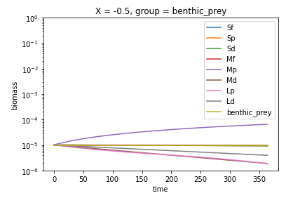
Michael Levy (Jan 12 2022 at 22:39):Matt and I worked out the last of the major kinks, and now my plot from the first column looks like this:
biomass-from-python-take-2.png
This is close to @Colleen Petrik's plot, but doesn't have Ld starting to grow in the middle of the year. Any hints on what to look for to figure out why that isn't being triggered? Here are the differences in biomass after the first time step:
| group | Matlab Value | Python Value | Rel Err |
|---|---|---|---|
| Sf | 9.9993e-06 | 9.9993e-06 | 8.1225e-06 |
| Sp | 9.9978e-06 | 9.9978e-06 | 5.7341e-08 |
| Sd | 9.9978e-06 | 9.9978e-06 | 5.7341e-08 |
| Mf | 1.1076e-05 | 1.1068e-05 | 7.0402e-04 |
| Mp | 1.1076e-05 | 1.1075e-05 | 4.7476e-05 |
| Md | 1.1030e-05 | 1.1030e-05 | 2.6002e-05 |
| Lp | 1.0093e-05 | 1.0094e-05 | 9.0167e-05 |
| Ld | 9.9746e-06 | 9.9745e-06 | 7.1689e-06 |
| benthic_prey | 2.0985e-03 | 2.0985e-03 | 2.4576e-05 |
Matt Long (Jan 12 2022 at 22:49):Getting there! This is great.
Matt Long (Jan 12 2022 at 22:49):why does Ld start to grow mid-year in @Colleen Petrik's runs? Are we sure that the forcing is the same?
Michael Levy (Jan 12 2022 at 22:55):I want to double check all of the input data (forcing, initial conditions, parameters, etc). I think something is slightly off in one (or more) of them, since the differences we're seeing in the first time step are much bigger than round-off. I was hoping the table above would show relative errors that were O(1e-10)...
Michael Levy (Jan 13 2022 at 21:02):It looks like the forcing data for the python code matches what is in the matlab code, but I think there's an off-by-one error in choosing which time level from the forcing to apply. Here's some forcing data from the first column for two days of a matlab run:
poc_flux: 0.02784712404856
T_pelagic: 18.20000000000000
T_bottom: 4.20000000000000

poc_flux: 0.02784643640657
T_pelagic: 18.19937772467829
T_bottom: 4.19997036784182
and the same output from python
poc_flux 0.027846436406572337
T_pelagic 18.19937772467829
T_bottom 4.199970367841823

poc_flux 0.027844373684374066
T_pelagic 18.19751108310676
T_bottom 4.199881480147941
Looks like there was a mismatch in time between the driver (1 -> 365) and the idealized forcing (0 -> 365)... I fixed that, and am now noticing an issue in T_habitat for Ld that is propagating through the computation but I think that's the last real issue. These encounter rates (aside from Ld_*) are much closer to what I expected:
| feeding_link | Matlab Value | Python Value | Rel Err |
|---|---|---|---|
| Sf_Zoo | 2.2885e+00 | 2.2885e+00 | 0.0000e+00 |
| Sp_Zoo | 2.2885e+00 | 2.2885e+00 | 0.0000e+00 |
| Sd_Zoo | 2.2885e+00 | 2.2885e+00 | 0.0000e+00 |
| Mf_Zoo | 2.9714e-01 | 2.9714e-01 | 1.8682e-16 |
| Mf_Sf | 1.9837e-06 | 1.9837e-06 | 0.0000e+00 |
| Mf_Sp | 1.9837e-06 | 1.9837e-06 | 0.0000e+00 |
| Mf_Sd | 1.9837e-06 | 1.9837e-06 | 0.0000e+00 |
| Mp_Zoo | 2.9714e-01 | 2.9714e-01 | 1.8682e-16 |
| Mp_Sf | 1.9837e-06 | 1.9837e-06 | 0.0000e+00 |
| Mp_Sp | 1.9837e-06 | 1.9837e-06 | 0.0000e+00 |
| Mp_Sd | 1.9837e-06 | 1.9837e-06 | 0.0000e+00 |
| Md_benthic_prey | 1.7232e-04 | 1.7232e-04 | 1.5729e-16 |
| Lp_Mf | 2.8618e-07 | 2.8618e-07 | 0.0000e+00 |
| Lp_Mp | 5.7237e-07 | 5.7237e-07 | 0.0000e+00 |
| Lp_Md | 0.0000e+00 | 0.0000e+00 | 0.0000e+00 |
| Ld_Mf | 8.9267e-08 | 8.9590e-08 | 3.6130e-03 |
| Ld_Mp | 1.7853e-07 | 1.7918e-07 | 3.6130e-03 |
| Ld_Md | 2.3805e-07 | 2.3891e-07 | 3.6130e-03 |
| Ld_benthic_prey | 4.9955e-05 | 5.0135e-05 | 3.6130e-03 |
Colleen Petrik (Jan 13 2022 at 23:22):Glad you found the time error, @Michael Levy . The reason that Ld doesn't grow until ~50 d is because there is zero recruitment into Ld until then. That is because the energy available for growth out of Md is negative before that time. @Matt Long
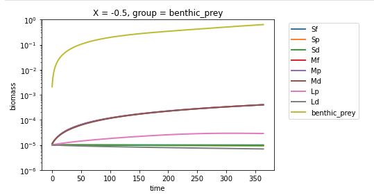
Michael Levy (Jan 13 2022 at 23:22):Okay, as of 0b646b7 I think most of the major bugs are squashed. Comparing to the matlab code, I'm seeing roundoff level differences in biomass after day 365:
| group | Matlab Value | Python Value | Rel Err |
|---|---|---|---|
| Sf | 1.7696e-05 | 1.7696e-05 | 3.8292e-16 |
| Sp | 9.3653e-06 | 9.3653e-06 | 0.0000e+00 |
| Sd | 9.4480e-06 | 9.4480e-06 | 0.0000e+00 |
| Mf | 4.0856e-04 | 4.0856e-04 | 1.3269e-16 |
| Mp | 3.1926e-04 | 3.1926e-04 | 3.3960e-16 |
| Md | 3.1755e-04 | 3.1755e-04 | 1.7071e-16 |
| Lp | 4.7386e-04 | 4.7386e-04 | 4.5760e-16 |
| Ld | 2.2672e-04 | 2.2672e-04 | 1.1955e-16 |
| benthic_prey | 6.3447e-01 | 6.3447e-01 | 0.0000e+00 |
The full-year plot looks pretty good, if I do say so myself:
biomass-from-python-take-3.png
I need to take off, but tomorrow morning I'll clean up open up issue tickets for all the issues I came across, link them to the PR, and then open the PR for review
Matt Long (Jan 13 2022 at 23:24):Terrific! Excellent work @Michael Levy!
Super excited to have achieved this milestone!
Michael Levy (Jan 14 2022 at 16:41):@Matt Long I think marbl-ecosys/feisty#6 is ready for review / merging... it's failing the documentation CI task because I don't know what I need to do to set things up so that I can push to the gh-pages branch from the VM but everything else should be passing and you probably got a dozen emails about the new issues I created / linked to the PR. (Fun fact; you can only link 10 issues to a PR, but that turned out to be exactly the number I needed.)
Matt Long (Jan 14 2022 at 19:22):I added you as admin on the project: maybe that will avoid this error in the future?
Michael Levy (Jan 14 2022 at 19:27):well, it looks like I didn't pay close attention to the CI results and broke test_simulate_testcase_init_2 -- so I'll see if the documentation builds for me after pushing a fix for that
Matt Long (Jan 14 2022 at 19:27):oh, I missed that too...and just merged
Michael Levy (Jan 14 2022 at 19:30):no worries, I'll throw together another branch
Colleen Petrik (Jan 21 2022 at 20:36):@Michael Levy , I created a new testcase with the Matlab code. It is in my fish-offline/MatFEISTY git repo. The main code is "test_locs3.m" and in the input files folder is a forcing file "feisty_input_climatol_daily_locs3" both in netcdf and mat format.
Michael Levy (Jan 21 2022 at 21:31):@Colleen Petrik thanks, that's great! I've opened up a PR (marbl-ecosys/feisty#24] where we apply the biomass tendency for benthic prey at the same time as the biomass tendency for fish in the python code. I know we talked about getting the same change into the matlab code -- do you want me to try to put together a similar pull request for fish-offline?
Colleen Petrik (Jan 21 2022 at 23:03):@Michael Levy , I changed the placement of the "sub_update_be" function to the end of "sub_futbio" Matlab code with the rest of the fish and pushed it. It does not appear to change the results of the 3 location test run.
Michael Levy (Jan 21 2022 at 23:06):thanks! I'm a little surprised that it doesn't change answers, but I'll update my checkout of fish-offline and then try to set up the three location test in python
Michael Levy (Jan 28 2022 at 21:45):@Colleen Petrik I needed to make one small change to sub_futbio_1meso.m to make sure we were updating the benthic prey biomass before any of the fish biomass (otherwise we were using the newly-updated Md.bio and Ld.bio instead of the values used elsewhere in the time-step):
$ git diff sub_futbio_1meso.m
diff --git a/MatFEISTY/sub_futbio_1meso.m b/MatFEISTY/sub_futbio_1meso.m
index 2091184..eb95e49 100644
--- a/MatFEISTY/sub_futbio_1meso.m
+++ b/MatFEISTY/sub_futbio_1meso.m
@@ -198,6 +198,8 @@ Ld.rec = sub_rec(Md.gamma,Md.bio);
 [Ld.bio, Ld.caught, Ld.fmort] = sub_fishing_rate(Ld.bio,param.dfrate,param.LDsel);

 % Mass balance
+[BENT.mass,BENT.pred] = sub_update_be(BENT.mass,param,ENVR.det,[Md.con_be,Ld.con_be],[Md.bio,Ld.bio]);
+
 Sf.bio = sub_update_fi(Sf.bio,Sf.rec,Sf.nu,Sf.rep,Sf.gamma,Sf.die,Sf.nmort,Sf.fmort);
 Sp.bio = sub_update_fi(Sp.bio,Sp.rec,Sp.nu,Sp.rep,Sp.gamma,Sp.die,Sp.nmort,Sp.fmort);
 Sd.bio = sub_update_fi(Sd.bio,Sd.rec,Sd.nu,Sd.rep,Sd.gamma,Sd.die,Sd.nmort,Sd.fmort);
@@ -209,8 +211,6 @@ Md.bio = sub_update_fi(Md.bio,Md.rec,Md.nu,Md.rep,Md.gamma,Md.die,Md.nmort,Md.fm
 Lp.bio = sub_update_fi(Lp.bio,Lp.rec,Lp.nu,Lp.rep,Lp.gamma,Lp.die,Lp.nmort,Lp.fmort);
 Ld.bio = sub_update_fi(Ld.bio,Ld.rec,Ld.nu,Ld.rep,Ld.gamma,Ld.die,Ld.nmort,Ld.fmort);

-[BENT.mass,BENT.pred] = sub_update_be(BENT.mass,param,ENVR.det,[Md.con_be,Ld.con_be],[Md.bio,Ld.bio]);
-
 % Forward Euler checks for demographics and movement
 Sf.bio=sub_check(Sf.bio);
 Sp.bio=sub_check(Sp.bio);
Without that change, benthic prey biomass differs between the matlab and python code and that spreads throughout the results with longer runs. With the above change, the python matches test_case.m to within roundoff after 1 year. E.g. here's the biomass comparison after a year:
| group | Matlab Value | Python Value | Rel Err |
|---|---|---|---|
| Sf | 1.7696e-05 | 1.7696e-05 | 0.0000e+00 |
| Sp | 9.3653e-06 | 9.3653e-06 | 0.0000e+00 |
| Sd | 9.4481e-06 | 9.4481e-06 | 0.0000e+00 |
| Mf | 4.0856e-04 | 4.0856e-04 | 1.3269e-16 |
| Mp | 3.1926e-04 | 3.1926e-04 | 0.0000e+00 |
| Md | 3.1755e-04 | 3.1755e-04 | 1.7071e-16 |
| Lp | 4.7386e-04 | 4.7386e-04 | 0.0000e+00 |
| Ld | 2.2687e-04 | 2.2687e-04 | 7.1683e-16 |
| benthic_prey | 6.3646e-01 | 6.3646e-01 | 0.0000e+00 |
Michael Levy (Jan 28 2022 at 21:47):Now I'm going to focus on getting the forcing from the new test_locs3.m into the python code... hopefully I'll have results early next week
Colleen Petrik (Jan 28 2022 at 21:59):Good catch, @Michael Levy ! I will update my local code and push it to git.
Michael Levy (Jan 28 2022 at 23:23):I've put in hooks to read forcing data from netCDF -- it's pretty kludgy, but at least it's reading the file. I think there might be differences between the netCDF and what the matlab code is producing, though:
| Matlab Value | Python Value | Rel Err | |
|---|---|---|---|
| T_pelagic | 4.7453e+00 | 4.7453e+00 | 2.3927e-09 |
| T_bottom | 4.7647e+00 | 4.7647e+00 | 3.3720e-08 |
| zooC | 7.0175e+00 | 7.0175e+00 | 2.7658e-09 |
| poc_flux_bottom | 0.0000e+00 | -7.8530e-03 | -inf |
| zoo_mort | 5.2470e-02 | 5.2470e-02 | 1.8489e-08 |
I need to take off, mostly leaving this comment so I know where to pick back up on Monday :) poc_flux_bottom looks concerning, and it would be nice to get the rest of the fields within O(1e-14) but O(1e-8) should be fine for initial testing
Michael Levy (Feb 03 2022 at 00:38):It looks like a few things were happening: (1) netcdf file was writing single precision instead of double, and (2) negative values of zooC, poc_flux_bottom, and zoo_mort were not being zeroed out. I regenerated the forcing file and that table is all 0s in the Rel Err column now. Unfortunately, I'm getting all nans in biomass after the first day, so clearly something else is going wrong - will investigate tomorrow
Michael Levy (Feb 03 2022 at 17:15):A few updates:
sub_futbio_1meso()nans in the biomass was due to the time dimension starting at 1 instead of 0Biomass from the python run looks really close to the matlab code after a full year:
| group | Matlab Value | Python Value | Rel Err |
|---|---|---|---|
| Sf | 1.3654e-05 | 1.3654e-05 | 0.0000e+00 |
| Sp | 9.5706e-06 | 9.5706e-06 | 0.0000e+00 |
| Sd | 1.0002e-05 | 1.0002e-05 | 1.6937e-16 |
| Mf | 2.4689e-04 | 2.4689e-04 | 2.1957e-16 |
| Mp | 2.1750e-04 | 2.1750e-04 | 0.0000e+00 |
| Md | 2.1868e-04 | 2.1868e-04 | 0.0000e+00 |
| Lp | 3.0769e-04 | 3.0769e-04 | 1.7618e-16 |
| Ld | 4.0795e-04 | 4.0795e-04 | 0.0000e+00 |
| benthic_prey | 2.8417e+01 | 2.8417e+01 | 1.6253e-15 |
I'm going to try running the full 20 years, but I think it'll take an hour or so to complete so I need to hop on a compute node...
Michael Levy (Feb 03 2022 at 17:16):to be clear, the above table is comparing biomass in the first column of the test_locs3.m setup after 1 year of simulation
Colleen Petrik (Feb 04 2022 at 01:40):@Michael Levy , this is great! I've been meaning to document the process for running FEISTY with any ESM or GCM output for you and @Matt Long :
In "make_grid_data_cesm_nonans.m" and similar
1a. Get model grid info on: Lon, Lat, Depth, Area, and ocean cells
1b. Save full those variables in 2D and extracted vector of ocean cells (1D) for each variable
In "daily_interp_cesm_fosi.m" and similar
2a. Convert forcing data from netcdf to units used in FEISTY (gWW/m2 for biomass or gWW/m2/d for fluxes/rates)
2b. Extract vector of each variable at the ocean cells
2c. Interpolate all forcing data from monthly to daily
Michael Levy (Feb 07 2022 at 22:22):I modified the matlab code to write out netCDF files instead of printing values to stdout and copying them into a YAML file... and it looks like the original 22 column idealized test case has some big differences outside of the first column:
| group | Matlab Value | Python Value | Rel Err |
|---|---|---|---|
| Sf (t=0, X=6) | 9.9993e-06 | 9.9993e-06 | 2.1013e-09 |
| Sp (t=0, X=0) | 9.9978e-06 | 9.9978e-06 | 0.0000e+00 |
| Sd (t=0, X=0) | 9.9978e-06 | 9.9978e-06 | 0.0000e+00 |
| Mf (t=0, X=6) | 1.1076e-05 | 1.1076e-05 | 4.0735e-09 |
| Mp (t=0, X=6) | 1.1076e-05 | 1.1076e-05 | 4.5556e-09 |
| Md (t=0, X=6) | 1.1030e-05 | 1.1030e-05 | 2.1251e-07 |
| Lp (t=0, X=6) | 1.0093e-05 | 1.0093e-05 | 4.2030e-07 |
| Ld (t=0, X=6) | 9.9746e-06 | 9.9402e-06 | 3.4473e-03 |
| benthic_prey (t=0, X=21) | 2.1760e-03 | 2.1760e-03 | 2.1544e-07 |
This is running for a single time step; I need to verify that the column depths and such match, and then I'll try to dig in to the individual components that make up the biomass computation to see if I can figure out what is causing these diffs
Michael Levy (Feb 07 2022 at 23:16):Okay, I think I fixed the above issue with
diff --git a/feisty/core/process.py b/feisty/core/process.py
index 4b9da4c..7b2c491 100644
--- a/feisty/core/process.py
+++ b/feisty/core/process.py
@@ -60,7 +60,7 @@ def compute_t_frac_pelagic(
             t_frac_pelagic[i, :] = xr.where(
                 domain.ocean_depth < PI_be_cutoff,
                 prey_pelagic / (prey_pelagic + prey_demersal),
-                1.0,
+                0.0,
             )
Does this make sense? If we're deeper than the Benthic-pelagic coupling cutoff, t_frac_pelagic is 0 instead of 1?
Michael Levy (Feb 07 2022 at 23:19):biomass comparison from the idealized testcase with the above fix:
| group | Matlab Value | Python Value | Rel Err |
|---|---|---|---|
| Sf (t=266, X=4) | 1.3672e-05 | 1.3672e-05 | 2.4781e-16 |
| Sp (t=0, X=0) | 9.9978e-06 | 9.9978e-06 | 0.0000e+00 |
| Sd (t=0, X=0) | 9.9978e-06 | 9.9978e-06 | 0.0000e+00 |
| Mf (t=263, X=4) | 2.5706e-04 | 2.5706e-04 | 2.1088e-16 |
| Mp (t=193, X=4) | 1.7676e-04 | 1.7676e-04 | 3.0669e-16 |
| Md (t=320, X=19) | 1.7271e-04 | 1.7271e-04 | 4.7083e-16 |
| Lp (t=157, X=4) | 1.4652e-04 | 1.4652e-04 | 5.5499e-16 |
| Ld (t=349, X=5) | 4.0468e-05 | 4.0468e-05 | 4.3537e-15 |
| benthic_prey (t=290, X=4) | 2.9726e-01 | 2.9726e-01 | 2.6144e-15 |
and for the 3-location test:
| group | Matlab Value | Python Value | Rel Err |
|---|---|---|---|
| Sf (t=298, X=0) | 1.2378e-05 | 1.2378e-05 | 2.7371e-16 |
| Sp (t=0, X=0) | 9.9989e-06 | 9.9989e-06 | 0.0000e+00 |
| Sd (t=0, X=0) | 9.9989e-06 | 9.9989e-06 | 0.0000e+00 |
| Mf (t=61, X=0) | 4.1794e-05 | 4.1794e-05 | 3.2427e-16 |
| Mp (t=4, X=2) | 1.5865e-05 | 1.5865e-05 | 2.1356e-16 |
| Md (t=258, X=0) | 1.5325e-04 | 1.5325e-04 | 3.5373e-16 |
| Lp (t=187, X=2) | 3.0789e-04 | 3.0789e-04 | 3.5214e-16 |
| Ld (t=214, X=1) | 2.0739e-05 | 2.0739e-05 | 1.7971e-15 |
| benthic_prey (t=327, X=1) | 2.9618e-01 | 2.9618e-01 | 1.6868e-15 |
Colleen Petrik (Feb 10 2022 at 20:31):@Michael Levy In the configuration I use that assumes large pelagic fish are pelagic specialists, t_frac_pelagic = 1 for SF, MF, SP, MP, LP, SD always; and t_frac_pelagic = 0 for MD always. The Benthic-Pelagic cutoff only matters for LD. So if we're deeper than the Benthic-pelagic coupling cutoff, t_frac_pelagic is 0, otherwise the prey densities are used to calculate it.
Michael Levy (Feb 10 2022 at 20:32):@Colleen Petrik -- perfect! In the python code, Ld is the only fish that calls compute_t_frac_pelagic() and the change I made was to set t_frac_pelagic = 0 if the column is deeper than the cutoff because the original code was setting it to 1 in those cases.
Michael Levy (Apr 01 2022 at 03:36):A status update, though plots won't be ready until tomorrow -- I updated the python code to accept monthly forcing instead of daily, and since the forcing is from mid-month the first 16 days will use the "12:00p on January 16th" values rather than extrapolating from the mid-January and mid-February values. So I expect the python solution to be similar to the matlab solution, but not within round-off. Some first tests seem to bear that out, but when I was trying to get the two to match closely I had modified the time axis to match what matlab uses when it does the interpolation to generate the daily forcing (30 day intervals, starting on day 15 rather than true mid-month).
For the interpolation, what I ended up doing is adding a _forcing_time to the offline driver class that is the first time level in the forcing when that is later than self.time, the last forcing level when that is earlier than self.time, and self.time everywhere else:
          self._forcing_time = np.where(
            self.time > self.forcing["time"].data[0],
            self.time,
            self.forcing["time"].data[0],
            )
          self._forcing_time = np.where(
            self._forcing_time < self.forcing["time"].data[-1],
            self._forcing_time,
            self.forcing["time"].data[-1]
The interpolation at time step n is then gcm_data_t = self.forcing.interp(time=forcing_t), where forcing_t = self._forcing_time[n].
The last thing to do before committing these changes is to update the default settings so they match the FOSI case (I'll use settings_in for the other test cases). Once that's done, it'll be time to turn to performance. I don't want to try to run the FOSI spin-up when it's taking 90 minutes per year (16 SYPD).
Michael Levy (Apr 01 2022 at 03:39):Looking at the code snippet, I think I should change the API of _compute_tendency so the call is dsdt = self._compute_tendency(n, state_t) instead of dsdt = self._compute_tendency(self.time[n], self._forcing_time[n], state_t)... so pretend that's already in place :)
Michael Levy (Apr 01 2022 at 16:05):@Colleen Petrik and @Matt Long -- As mentioned in my last post, there are a couple of differences in how the python and matlab code handle forcing:
With these differences is mind, I ran one year using the first year of FOSI forcing. The intial conditions were spun-up by repeating this forcing for 150 or 200 years, so the expectation is that the system is close to equilibrium.
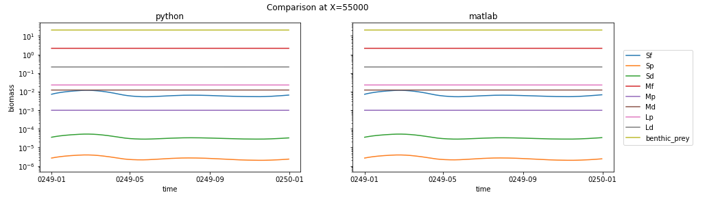
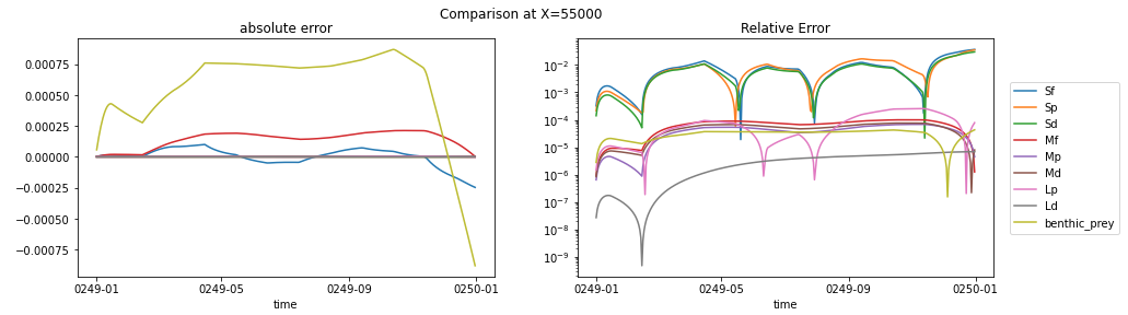
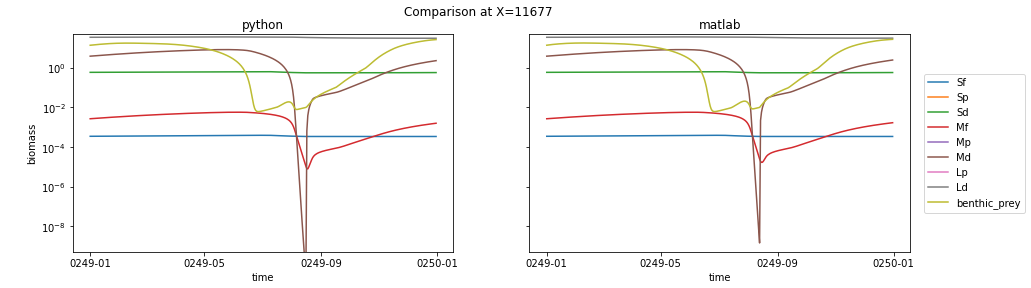
I picked two grid cells to plot biomass from, one where the the two model solutions look pretty similar and one where there are clear differences. Here's the side-by-side comparison of what I think is a sign that the two models are behaving similarly (I picked this point because I was looking for (a) biomass values larger than 1e-7 in all groups, and (b) small differences between python and matlab):
Here are the absolute and relative errors at the same point:
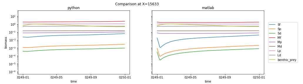
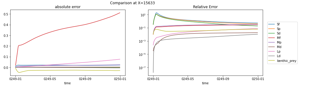
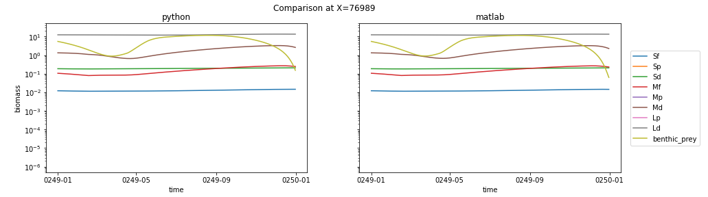
For the column showing differences between the two, I looked at the grid cell reporting the largest relative error for Sf, Sp, and Sd (probably not a coincidence that all three maximums occur in the same location). Here's the side-by-side of biomass:
and the error plots:
It's interesting to me that the three small classes all show a big drop early in the matlab run, followed by a recovery to the equilibrium state, while the python run stays in equilibrium. My take is that this is a response to the difference in interpolation techniques prior to Jan 15, but that all-in-all it's a sign that the python code is running well.
Michael Levy (Apr 01 2022 at 16:16):And two more plots, because I think they're interesting. biomass in the column with the biggest errors from the medium classes:
The error seems to be largest where the huge drop in Md (and smaller drop in Mf) occur. It would be interesting to find out what's causing the abrupt drop (and just as abrupt recovery).
Here's the column with the largest errors in the benthic prey:
It looks like there are only 6 classes plotted because Sp, Mp, and Lp are all order 1e-19 or so.
The column with the largest errors in the large class aren't very interesting (Lp is very small, and the error in Ld is roughly 1e-2)
Michael Levy (Apr 01 2022 at 20:47):I did a little profiling: about 82% of the python runtime is spent interpolating the forcing field (!!) and only ~8% is spent actually computing the tendency. It turns out an easy way to cut this down by a factor of 10 is to reduce the size of the time dimension from 68 years to 1 year... so I think a smart .isel(time=...) in gcm_data_t = self.forcing.interp(time=forcing_t) will be a big savings.
Michael Levy (Apr 01 2022 at 23:05):@Keith Lindsay helped find the assume_sorted flag in xarray's interp() function, and instead of 90+ minutes, I'm down to 7.5 minutes per year! (I think matlab is 1.5 minutes per year, so still 5x slower). Here's the latest timing data, without breaking down each call in compute_tendencies():
Elapsed time for init: 49.47
Elapsed time for post_data: 317.51
Elapsed time for interp_forcing: 9.55
Elapsed time for compute_tendency: 79.63
Elapsed time for solve: 456.21
Total (excluding solve, which wraps the rest): 456.15
CPU times: user 1min 41s, sys: 1min 47s, total: 3min 29s
Wall time: 7min 36s
init is copying the prognostic variables into state_t and setting up the arrays for output; post_data is copying state_t back into biomass and updating the diagnostics in the offline_driver object (so copying from one Dataset to another). I can look at speeding up that step next week
Matt Long (Apr 01 2022 at 23:59):@Michael Levy , this seems like a very good, important step. I am really concerned about the performance, however.
Michael Levy (Apr 02 2022 at 04:14):The post_data stage is clearly the next one to target, and I have a few ideas. Namely, could we avoid memory copies by doing intermediate computations directly into the diagnostic data arrays? I’ll look into it Monday
Michael Levy (Apr 04 2022 at 19:44):I was able to greatly reduce the time spent in post_data by not posting most of the diagnostic output:
Elapsed time for init: 35.61
Elapsed time for post_data: 15.64
Elapsed time for interp_forcing: 6.85
Elapsed time for compute_tendency: 62.31
Elapsed time for solve: 120.45
Total (excluding solve, which wraps the rest): 120.41
CPU times: user 1min 7s, sys: 36.1 s, total: 1min 43s
Wall time: 2min
So this is closer in line to matlab timing (90 seconds, but that excludes some of the matlab initialization), but the bulk of the savings comes about by not copying T_habitat, ingestion_rate, predation_flux, predation_rate, metabolism_rate', mortality_rate, energy_avail_rate, growth_rate, reproduction_rate, recruitment_flux, fish_catch_rate, encounter_rate_link, encounter_rate_total, consumption_rate_max_pred, or consumption_rate_link into a Dataset every time step... which means those diagnostics are not available after the run
Michael Levy (Apr 04 2022 at 19:46):Actually, the above timing just commented out the data copy into each time slice. If I actually remove the diagnostics from the dataset (e.g. don't initialize the memory for them), we actually meet the matlab performance numbers!
Elapsed time for init: 2.19
Elapsed time for post_data: 14.93
Elapsed time for interp_forcing: 6.89
Elapsed time for compute_tendency: 61.97
Elapsed time for solve: 86.02
Total (excluding solve, which wraps the rest): 85.98
CPU times: user 1min 3s, sys: 7.08 s, total: 1min 10s
Wall time: 1min 26s
I extended the above setup to a 50 year run (trying to do the FOSI spinup run, so forcing is just cycling over the first year), and the overhead is pretty large:
Elapsed time for init: 262.06
Elapsed time for post_data: 1750.98
Elapsed time for interp_forcing: 2588.41
Elapsed time for compute_tendency: 9191.34
Elapsed time for solve: 13801.51
Total (excluding solve, which wraps the rest): 13792.79
CPU times: user 1h 12min 17s, sys: 2h 9min 13s, total: 3h 21min 31s
Wall time: 3h 50min 1s
It's nice to see the 1-year run in the 90-second range, but I really want to maintain that throughput for longer runs. The numbers above average out to ~270 seconds / year, or 3x slower, and I assume it boils down to memory management because we are allocating a ton of memory upfront.
I'm thinking about refactoring the offline driver to do everything in one-year chunks (like the matlab code)... I'm picturing a cycle of
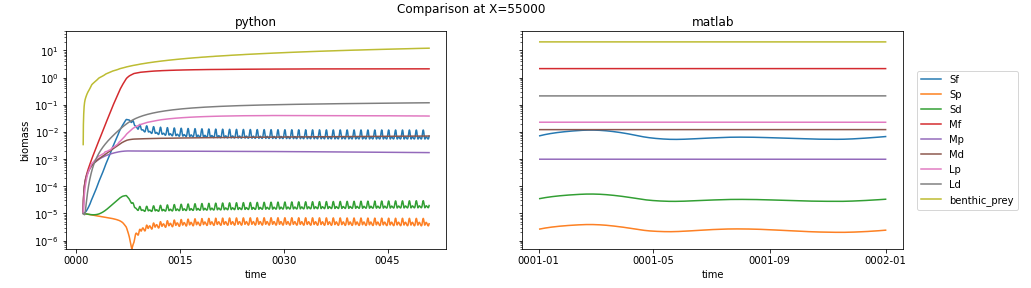
xr.concat()The good news is that the results look promising. Here's a time series of biomass over the full 50 years at one of the columns I've been using to check my run, with one year of the already-spun-up matlab output for comparison:
50-year-spinup-compared-to-spun-up-matlab.png
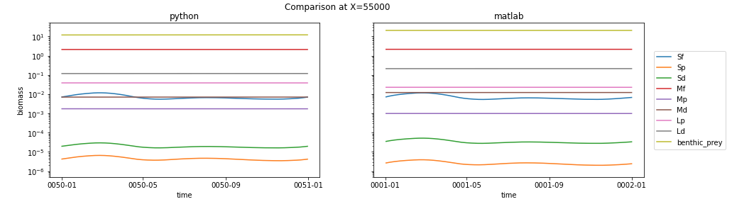
And then here is the last year of the spinup from the same column (with the same matlab plot for comparison):
50th-year-of-spinup-compared-to-spun-up-matlab.png
The big differences to my eye are
Sd, Md, and Ld are a little lower in the python run than the matlab, while Sp, Mp, and Lp are a little higher (much more noticeable in Lp, Ld, and Md than the other three fields) Matt Long (Apr 05 2022 at 17:05):I think you're plan regarding running year-by-year sounds reasonable, though I think you might be able to simply dump the data at some prescribed (i.e., annual) frequency in context of the time loop, rather than hard coding a model stop/start.
Michael Levy (Apr 05 2022 at 17:52):My hope is to preserve the the testcase.run(nt) interface, I was just picturing a loop under the covers to make sure we don't exceed bounds when copying into the numpy arrays. "Dumping output" (maybe just creating a list of datasets that a user can merge after the fact?) makes sense, and maybe we could work that in without really messing with anything else in _solve()
Matt Long (Apr 05 2022 at 18:58):I was thinking that if the conditional is met (i.e., time to write out a file), the index into the memory buffer could be reset and the time-stepping loop could just proceed. So something like time_step_per_file could be set... Another issues relates to temporal averaging. We are still writing time-step level output, right? Ideally we would decouple the timestep from the output frequency and enable temporal averaging. Not clear to me that this is a priority.
Michael Levy (Apr 05 2022 at 21:30):Okay, I broke self._ds into a list of datasets with a max length of self._max_output_time_dim (default set to 365, and I haven't tried adjusting it); this lets the model run much faster, but requires an xr.concat() at the end which can be time consuming. Bottom line, the 50-year run that took 3 hours 50 minutes last night is down to an hour and a half (so 108 seconds per year)
Matt Long (Apr 06 2022 at 12:59):that seems reasonable. I think if we write single var files, the concat step can be skipped...but that's a detail. Parallelization should make dramatic gains in performance.
Colleen Petrik (May 25 2022 at 21:37):@Michael Levy , why are the netcdf files so large? For example, the 4yr FOSI file we created today is 9.02GB, while my netcdfs from the Matlab version for the full 62 years of the FOSI are 10.08GB.
Michael Levy (May 25 2022 at 21:38):whoa, that's a big difference. I think we're spitting stuff out in double precision, while matlab might be writing single precision, but that would only be a factor of 2
Michael Levy (May 25 2022 at 21:40):but there are 9 functional types, and 85000 grid cells, so 1 year (365 daily output) would be 8*9*85000*365 = 2.2 billion bytes per year... maybe matlab is writing compressed netcdf?
Michael Levy (May 25 2022 at 21:41):I did notice that my 62 year FOSI run created a 110GB netcdf file, and that seemed a little extreme...
Colleen Petrik (May 26 2022 at 00:27):Yes, that's a bit extreme! I realized the difference is that I save monthly means, not daily.
Michael Levy (May 26 2022 at 15:27):I can add a flag to the settings file to compute monthly means, that should be pretty easy with xarray
Last updated: May 16 2025 at 17:14 UTC