
Examine History Files#
Having successfully completed your first month of the new CLM I1850sp case, you will now examine the history files that have been transfered to the Archive directory. You will be using the NetCDF viewer ncvis to look at the monthly average values for the single month. In this exercise we will:
Step 1. Explore the i1850sp.basics Archive directory.
Step 2. Open the i1850sp.basics CLM monthly history file using ncvis.
Step 3. Examine Average Monthly 2m Air Temperature (TSA).
Step 4. Examine Instantaneous Snow Persistence.
Step 1. Explore the i1850sp.basics Archive directory#
The short term archive directory has a range of model component directories along with the restart (rest) and logs directories. First, change directory into the archive directory, and then list the contents of the restart and logs directories.
cd /glade/derecho/scratch/$USER/archive/i1850sp.basics
List the logs directory:
ls -l logs
This is where all the log files from the model run are stored.
List the logs directory:
ls -l rest/0001-02-01-00000
These are the files that clm will use to restart the model.
Step 2. Open the CLM h0 monthly average history files#
You will now use ncvis to look at the i1850sp.basics case CLM monthly average values for the single month you ran.
If you are unfamiliar with ncvis, you can learn more at this link.
Note: You must load the ncvis module to your environment. If you loaded the tutorial .profile or .tcshrc file it should already be loaded. Check that it is in your environment.
module list
If you don’t see ncvis in the list of modules, you can load it by doing:
module load ncvis
cd lnd/hist
List the files in the directory:
ls -l
There should be two files, i1850sp.basics.clm.h0a.0001-01.nc and i1850_sp.basics.clm2.h0i.0001-01.nc.
Open the h0a (average) file using ncvis:
ncvis i1850sp.basics.clm.h0a.0001-01.nc &
If your X11 environment is correctly set up, then the Ncvis tool should appear as shown below. It might be just a little slow to load. Note the & at the end of the command. This puts the command into the background, allowing other tasks to be run from the Derecho terminal window.
Figure: NCVis App Window 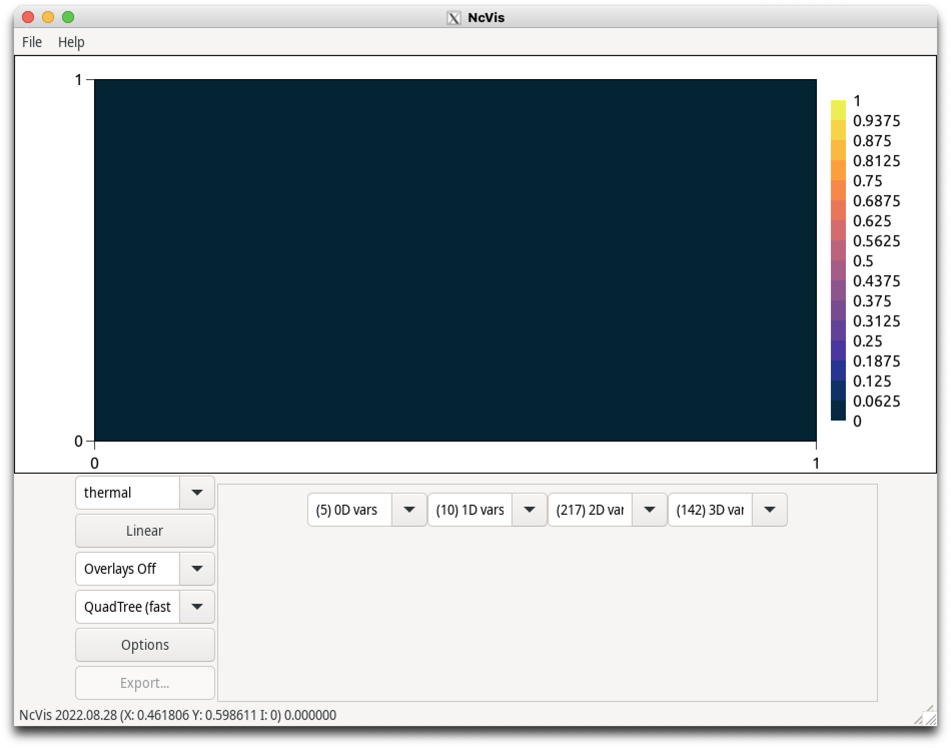
Step 3. Examine Average Monthly Average 2m Air Temperature#
Using Ncvis with the i1850sp.basics January 0001 CLM monthly average values file loaded, examine the 2m Air Temperature variable. Update the color palette used to plot values and change the size of the plot.
Click on the (365) 3D vars button shown above. This will pull up a list of all 3d vars on the i1850sp.basics January 0001 CLM average history file. This is a long list but it is in alphabetical order. You are looking for the TSA variable.
Change the color selection from detail to bright:
Clicking on the top left drop-down (that says “thermal” in the image above) will give a list of possible color maps for the contour plot. Choose another option to see how the color scale can change.
Add map overlays:
Click on the dropdown on the left side that says “Overlays off” by default. There should be two more options, “ne_110m_coastline.shp” and “ne_110m_admin_0_countries.shp”. Try clicking each of these and see how maps are added to your temperature plot.
The 2m Air Temperature variable is in Kelvin. A value of 273.15K represents 0°C and 32°F. As you move your mouse cursor over the map, you will see the location given (“X:” and “Y:”) in the lower left corner and the temperature value at the cursor point. There are many options to better view and explore data with Ncvis. Some of these will come up over the next few days of the tutorial.
Figure: NCVis i1850sp.basics Average TSA Jan 0001 with the Jet colorscale and map outlines 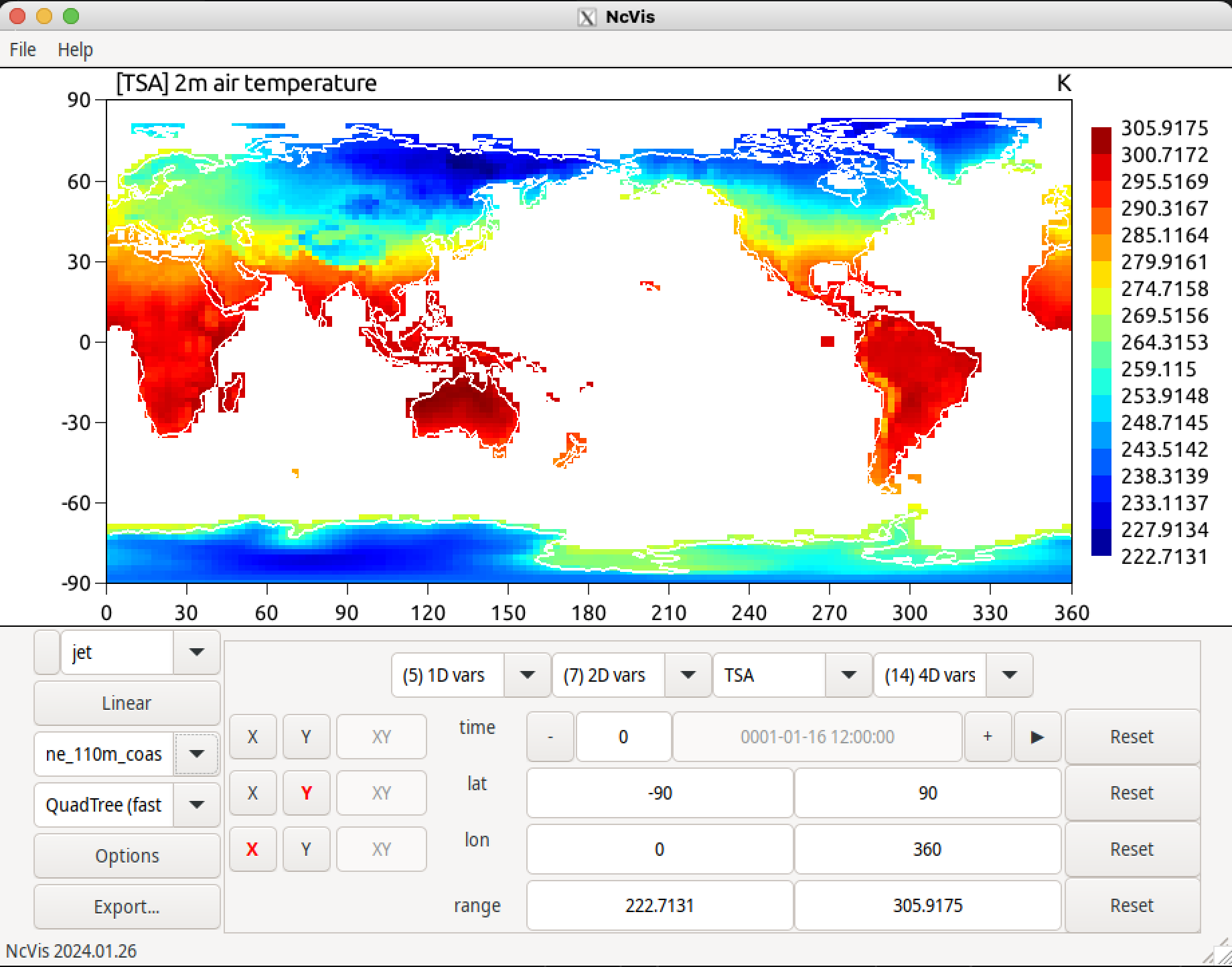
Step 4. Examine Instantaneous Snow Persistence#
Components in CESM generally seperate history fields into seperate files by their averaging type and timescale. In the land model, there are two history files by default. The “h0a” file holds fields averaged for the time period specified in the filename and file metadata. The “h0i” file hold instantaneous data from the timestep shown in the filename and the file metadata. In our basic example, the only field in the instantaneous file is for snow persistence “SNOW_PERSISTENCE”.
Open the h0i file using ncvis:
ncvis i1850_sp.basics.clm2.h0i.0001-01.nc &
Select the snow persistence variable:
Click on the (1) 3D vars button. Date written and Time written are metadata variables, but SNOW_PERSISTENCE can be plotted. Choose a colorscale and map overlay that you like.
Figure: NCVis i1850sp.basics Instantaneous snow persistence Jan 01 0001 with the Haline colorscale and map outlines 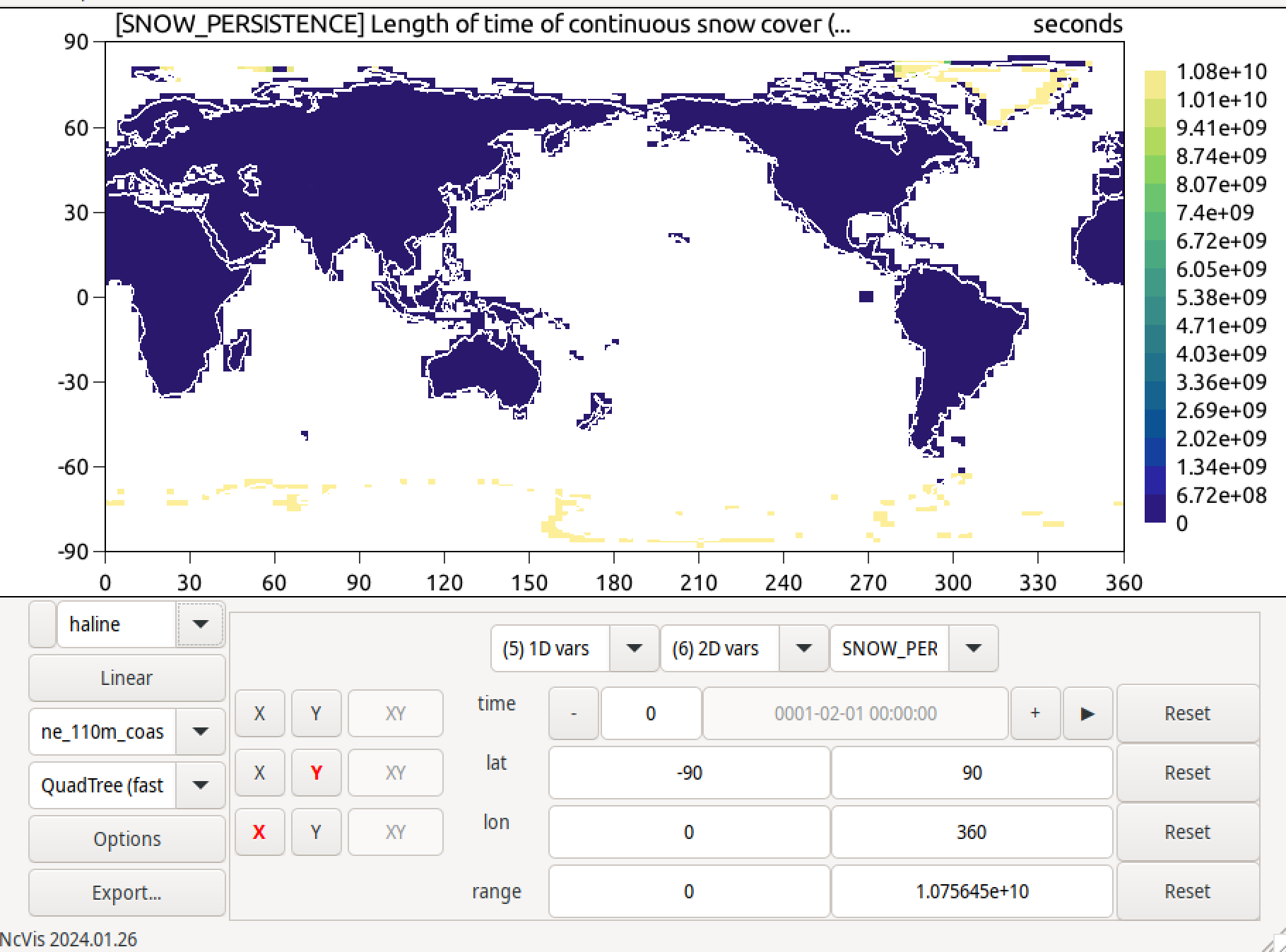
By default, there is only one variable and one time slice written to the h0i file each month for this configuration. Later exercises will describe how to add more instantaneous or averaged output, more time slices per file, and other history file options.