origin:ncar-posix origin:ncar-object-store platform:casper dataset:na-cordex task:visualization level:intermediate
This notebook is adapted from the NA CORDEX notebook on AWS
http://
ncar -aws -www .s3 -website -us -west -2 .amazonaws .com /plot -zarr -diagnostics .html
Input Data Access
This notebook illustrates how to make diagnostic plots using the NA-CORDEX dataset hosted on NCAR’s Geoscience Data Exchange (GDEX)
This data is open access and can be accessed via 2 protocols
HTTPS (if you have access to NCAR’s HPC)
OSDF using an intake-ESM catalog.
# Imports
import intake
import numpy as np
import pandas as pd
import xarray as xr
import seaborn as sns
import re
import matplotlib.pyplot as plt
import dask
from dask_jobqueue import PBSCluster
from dask.distributed import Client
import os
init_year0 = '1991'
init_year1 = '2020'
final_year0 = '2071'
final_year1 = '2100'# catalog_url = 'https://osdf-data.gdex.ucar.edu/ncar-gdex/d316010/catalogs/d316010-osdf-zarr.json'
catalog_url = 'https://osdata.gdex.ucar.edu/d316010/catalogs/d316010-osdf.json' #NCAR's Object store
print(catalog_url)https://osdata.gdex.ucar.edu/d316010/catalogs/d316010-osdf.json
# Set up your scratch folder path
username       = os.environ["USER"]
glade_scratch  = "/glade/derecho/scratch/" + username
print(glade_scratch)
/glade/derecho/scratch/harshah
Create a PBS cluster
# Create a PBS cluster object
cluster = PBSCluster(
    job_name = 'dask-wk24-hpc',
    cores = 1,
    memory = '8GiB',
    processes = 1,
    local_directory = glade_scratch+'/dask/spill',
    log_directory = glade_scratch + '/dask/logs/',
    resource_spec = 'select=1:ncpus=1:mem=8GB',
    queue = 'casper',
    walltime = '5:00:00',
    #interface = 'ib0'
    interface = 'ext'
)
/glade/u/home/harshah/.conda/envs/osdf/lib/python3.11/site-packages/distributed/node.py:188: UserWarning: Port 8787 is already in use.
Perhaps you already have a cluster running?
Hosting the HTTP server on port 34989 instead
warnings.warn(
# Create the client to load the Dashboard
client = Client(cluster)
n_workers = 8
cluster.scale(n_workers)
client.wait_for_workers(n_workers = n_workers)
cluster
Loading...
Load NA CORDEX data from GDEX using an intake catalog
col = intake.open_esm_datastore(catalog_url)
col
Loading...
Load data into xarray
data_var = 'tmax'

col_subset = col.search(
    variable=data_var,
    grid="NAM-44i",
    scenario="eval",
    bias_correction="raw",
)

col_subset
Loading...
col_subset.df['path'].values<ArrowExtensionArray>
['osdf:////ncar-gdex/d316010/day/tmax.eval.day.NAM-44i.raw.zarr']
Length: 1, dtype: large_string[pyarrow]col_subset['tmax.day.eval.NAM-44i.raw'].dfLoading...
# Load catalog entries for subset into a dictionary of xarray datasets, and open the first one.
dsets = col_subset.to_dataset_dict(zarr_kwargs={"consolidated": True,'zarr_format':2})
print(f"\nDataset dictionary keys:\n {dsets.keys()}")
--> The keys in the returned dictionary of datasets are constructed as follows:
	'variable.frequency.scenario.grid.bias_correction'
Loading...
Dataset dictionary keys:
 dict_keys(['tmax.day.eval.NAM-44i.raw'])
# Load the first dataset and display a summary.
dataset_key = list(dsets.keys())[0]
store_name = dataset_key + ".zarr"

ds = dsets[dataset_key]
ds
Loading...
Functions for Plotting
Helper Function to Create a Single Map Plot
def plotMap(ax, map_slice, date_object=None, member_id=None):
    """Create a map plot on the given axes, with min/max as text"""

    ax.imshow(map_slice, origin='lower')

    minval = map_slice.min(dim = ['lat', 'lon'])
    maxval = map_slice.max(dim = ['lat', 'lon'])

    # Format values to have at least 4 digits of precision.
    ax.text(0.01, 0.03, "Min: %3g" % minval, transform=ax.transAxes, fontsize=12)
    ax.text(0.99, 0.03, "Max: %3g" % maxval, transform=ax.transAxes, fontsize=12, horizontalalignment='right')
    ax.set_xticks([])
    ax.set_yticks([])

    if date_object:
        ax.set_title(date_object.values.astype(str)[:10], fontsize=12)

    if member_id:
        ax.set_ylabel(member_id, fontsize=12)

    return ax
Helper Function for Finding Dates with Available Data
def getValidDateIndexes(member_slice):
    """Search for the first and last dates with finite values."""
    min_values = member_slice.min(dim = ['lat', 'lon'])
    is_finite = np.isfinite(min_values)
    finite_indexes = np.where(is_finite)

    start_index = finite_indexes[0][0]
    end_index = finite_indexes[0][-1]
    return start_index, end_index
Function Producing Maps of First, Middle, and Final Timesteps
def plot_first_mid_last(ds, data_var, store_name):
    """Plot the first, middle, and final time steps for several climate runs."""
    num_members_to_plot = 4
    member_names = ds.coords['member_id'].values[0:num_members_to_plot]

    figWidth = 18
    figHeight = 12
    numPlotColumns = 3
    fig, axs = plt.subplots(num_members_to_plot, numPlotColumns, figsize=(figWidth, figHeight), constrained_layout=True)

    for index in np.arange(num_members_to_plot):
        mem_id = member_names[index]
        data_slice = ds[data_var].sel(member_id=mem_id)

        start_index, end_index = getValidDateIndexes(data_slice)
        midDateIndex = np.floor(len(ds.time) / 2).astype(int)

        startDate = ds.time[start_index]
        first_step = data_slice.sel(time=startDate)
        ax = axs[index, 0]
        plotMap(ax, first_step, startDate, mem_id)

        midDate = ds.time[midDateIndex]
        mid_step = data_slice.sel(time=midDate)
        ax = axs[index, 1]
        plotMap(ax, mid_step, midDate)

        endDate = ds.time[end_index]
        last_step = data_slice.sel(time=endDate)
        ax = axs[index, 2]
        plotMap(ax, last_step, endDate)

        plt.suptitle(f'First, Middle, and Last Timesteps for Selected Runs in "{store_name}"', fontsize=20)

    return fig
Function Producing Statistical Map Plots
def plot_stat_maps(ds, data_var, store_name):
    """Plot the mean, min, max, and standard deviation values for several climate runs, aggregated over time."""

    num_members_to_plot = 4
    member_names = ds.coords['member_id'].values[0:num_members_to_plot]

    figWidth = 25
    figHeight = 12
    numPlotColumns = 4

    fig, axs = plt.subplots(num_members_to_plot, numPlotColumns, figsize=(figWidth, figHeight), constrained_layout=True)

    for index in np.arange(num_members_to_plot):
        mem_id = member_names[index]
        data_slice = ds[data_var].sel(member_id=mem_id)

        data_agg = data_slice.min(dim='time')
        plotMap(axs[index, 0], data_agg, member_id=mem_id)

        data_agg = data_slice.max(dim='time')
        plotMap(axs[index, 1], data_agg)

        data_agg = data_slice.mean(dim='time')
        plotMap(axs[index, 2], data_agg)

        data_agg = data_slice.std(dim='time')
        plotMap(axs[index, 3], data_agg)

    axs[0, 0].set_title(f'min({data_var})', fontsize=15)
    axs[0, 1].set_title(f'max({data_var})', fontsize=15)
    axs[0, 2].set_title(f'mean({data_var})', fontsize=15)
    axs[0, 3].set_title(f'std({data_var})', fontsize=15)

    plt.suptitle(f'Spatial Statistics for Selected Runs in "{store_name}"', fontsize=20)

    return fig
Function Producing Time Series Plots
Also show which dates have no available data values, as a rug plot.
def plot_timeseries(ds, data_var, store_name):
    """Plot the mean, min, max, and standard deviation values for several climate runs,
       aggregated over lat/lon dimensions."""

    num_members_to_plot = 4
    member_names = ds.coords['member_id'].values[0:num_members_to_plot]

    figWidth = 25
    figHeight = 20
    linewidth = 0.5

    numPlotColumns = 1
    fig, axs = plt.subplots(num_members_to_plot, numPlotColumns, figsize=(figWidth, figHeight))

    for index in np.arange(num_members_to_plot):
        mem_id = member_names[index]
        data_slice = ds[data_var].sel(member_id=mem_id)
        unit_string = ds[data_var].attrs['units']

        min_vals = data_slice.min(dim = ['lat', 'lon'])
        max_vals = data_slice.max(dim = ['lat', 'lon'])
        mean_vals = data_slice.mean(dim = ['lat', 'lon'])
        std_vals = data_slice.std(dim = ['lat', 'lon'])

        missing_indexes = np.isnan(min_vals)
        missing_times = ds.time[missing_indexes]


        axs[index].plot(ds.time, max_vals, linewidth=linewidth, label='max', color='red')
        axs[index].plot(ds.time, mean_vals, linewidth=linewidth, label='mean', color='black')
        axs[index].fill_between(ds.time, (mean_vals - std_vals), (mean_vals + std_vals),
                                         color='grey', linewidth=0, label='std', alpha=0.5)
        axs[index].plot(ds.time, min_vals, linewidth=linewidth, label='min', color='blue')

        ymin, ymax = axs[index].get_ylim()
        rug_y = ymin + 0.01*(ymax-ymin)
        axs[index].plot(missing_times, [rug_y]*len(missing_times), '|', color='m', label='missing')
        axs[index].set_title(mem_id, fontsize=20)
        axs[index].legend(loc='upper right')
        axs[index].set_ylabel(unit_string)

    plt.tight_layout(pad=10.2, w_pad=3.5, h_pad=3.5)
    plt.suptitle(f'Temporal Statistics for Selected Runs in "{store_name}"', fontsize=20)

    return fig
Produce Diagnostic Plots
Plot First, Middle, and Final Timesteps for Several Output Runs (less compute intensive)
%%time
# Plot using the Zarr Store obtained from an earlier step in the notebook.
figure = plot_first_mid_last(ds, data_var, store_name)

plt.show()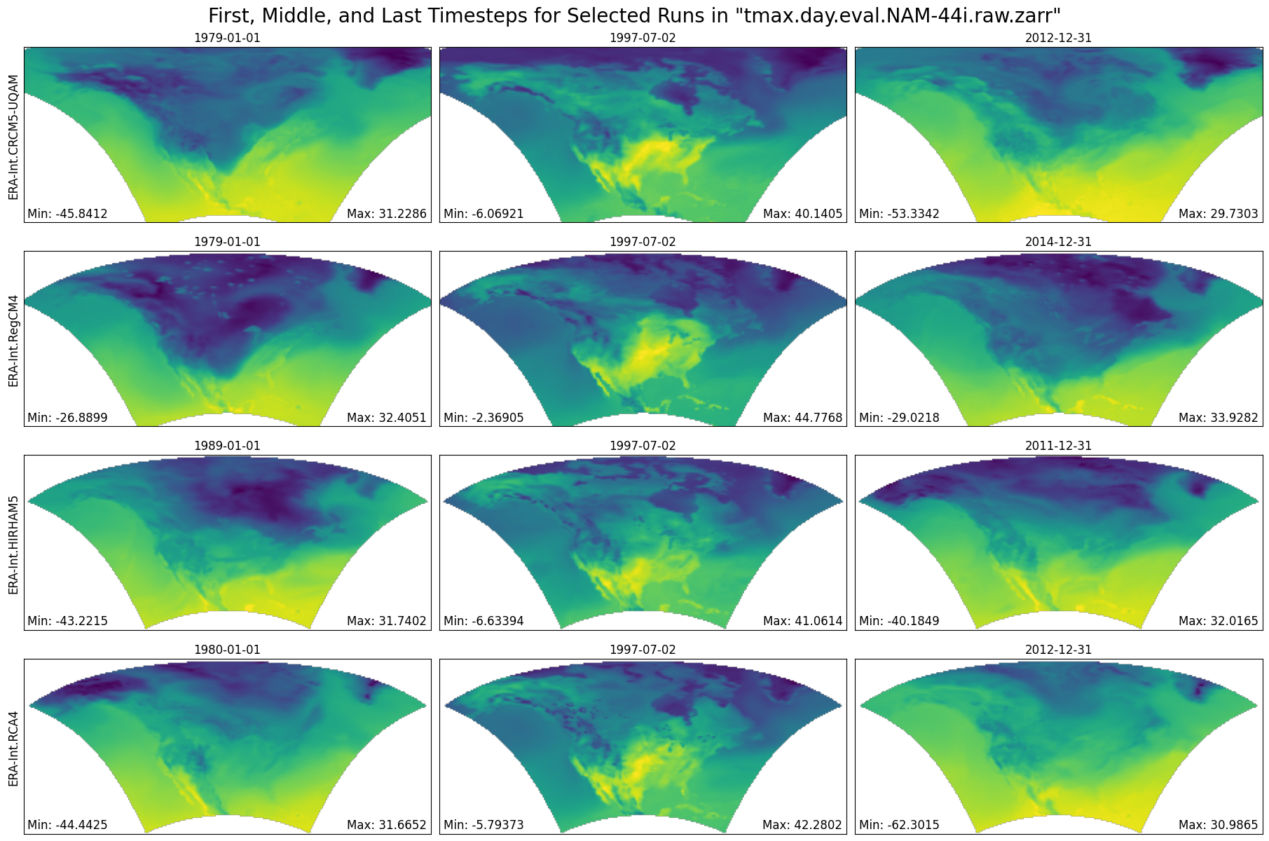
CPU times: user 2.48 s, sys: 221 ms, total: 2.7 s
Wall time: 44.7 s
cluster.close()