Plot Evolution

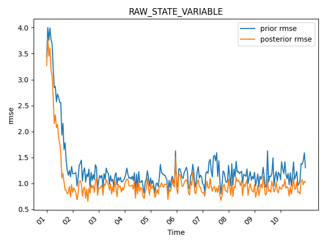
This example demonstrates how to plot the evolution of RMSE, bias, or totalspread. For an explanation of the statistics calculations see the Statistics guide.

Import the obs_sequence module and the matplots module for plotting.

import pydartdiags.obs_sequence.obs_sequence as obsq
from pydartdiags.matplots import matplots as mp

Chose an obs_seq file to read. In this example, we are using “obs_seq.final.lorenz_96” which is from a Lorenz 96 model run with the DART assimilation system. The obs_seq.final.lorenz_96 file comes with the pyDARTdiags package in the data directory, so we import os to get the path to the file.

import os
data_dir = os.path.join(os.getcwd(), "../..", "data")
data_file = os.path.join(data_dir, "obs_seq.final.lorenz_96")

Read the obs_seq file into an obs_seq object.

obs_seq = obsq.ObsSequence(data_file)

fig = mp.plot_evolution(
    obs_seq=obs_seq,
    type="RAW_STATE_VARIABLE",
    time_bin_width="3600s",  # 1-hour bins
    stat="rmse",
    tick_interval=24,
    time_format="%d", # days
    plot_pvu=False
)

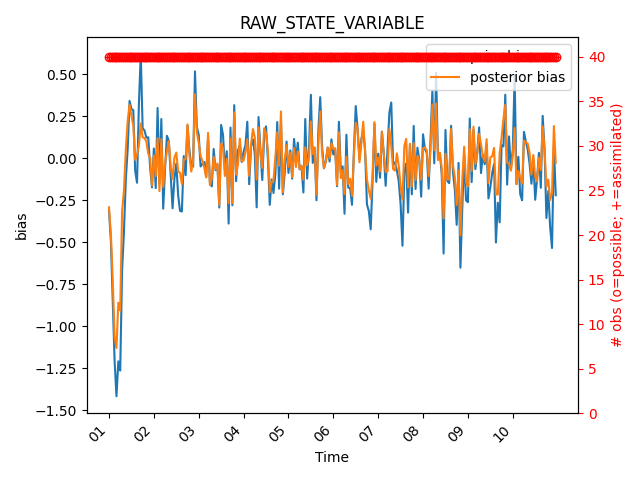
To plot the bias, set stat=”bias”. Let’s also plot the possible vs used observations.

fig = mp.plot_evolution(
    obs_seq=obs_seq,
    type="RAW_STATE_VARIABLE",
    time_bin_width="3600s",  # 1-hour bins
    stat="bias",
    tick_interval=24,
    time_format="%d", # days
    plot_pvu=True
)

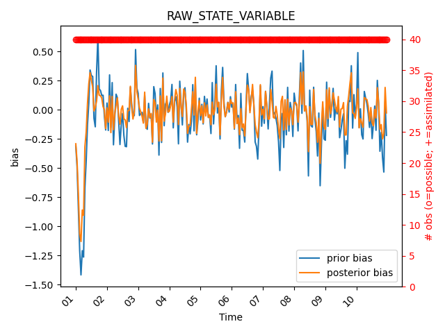
The legend is being covered by the ‘used vs. assimilated’ observation count, so let’s move the legend to the lower right corner. We can do this by accessing the matplotlib axes object from the figure and using the legend method to move the legend.

fig = mp.plot_evolution(
    obs_seq=obs_seq,
    type="RAW_STATE_VARIABLE",
    time_bin_width="3600s",  # 1-hour bins
    stat="bias",
    tick_interval=24,
    time_format="%d", # days
    plot_pvu=True
)

# Get the Axes object from the figure
ax = fig.axes[0]  # Axis 0 refers to the first Axes object

# Move the legend to a new location
legend = ax.legend(loc="lower right")