Regridding using xESMF and an existing weights file

A fairly common request is to use an existing ESMF weights file to regrid a Xarray Dataset (1, 2). Applying weights in general should be easy: read weights then apply them using dot or tensordot on the input dataset.

In the Xarray/Dask/Pangeo ecosystem, xESMF provides an interface to ESMF for convenient regridding, includiing parallelization with Dask. Here we demonstrate how to use an existing ESMF weights file with xESMF specifically for CAM-SE.

CAM-SE is the Community Atmosphere Model with the spectral element dynamical core (Dennis et al, 2011)

The spectral element dynamical core, CAM-SE, is an unstructured grid that supports uniform resolutions based on the equiangular gnomonic cubed-sphere grid as well as a mesh refinement capability with local increases in resolution through conformal mesh refinement. CAM-SE is the default resolution for CESM2 high resolution capabilities … (Lauritzen et al. 2018).

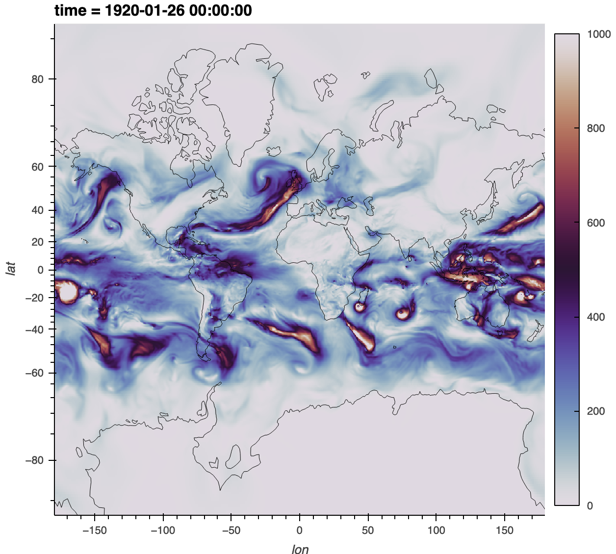
The main challenge is the input dataset has one spatial dimension (ncol), while xESMF is hardcoded to expect two spatial dimensions (lat, lon). We solve that by adding a dummy dimension. At the end, we’ll make this plot of the vertically integrated water vapour transport (IVT)

from IPython.display import Image

Image("../images/cam-se-ivt.png", width=600)

%load_ext watermark

import hvplot.xarray
import matplotlib.pyplot as plt
import numpy as np
import xarray as xr
import xesmf

%watermark -iv

sys       : 3.10.8 | packaged by conda-forge | (main, Nov 22 2022, 08:26:04) [GCC 10.4.0]
numpy     : 1.23.5
matplotlib: 3.6.2
xesmf     : 0.6.3
json      : 2.0.9
xarray    : 2022.12.0
hvplot    : 0.8.2

Read data

First some file paths

data_file = "/glade/campaign/collections/cmip/CMIP6/iHESP/BHIST/HR/b.e13.BHISTC5.ne120_t12.cesm-ihesp-hires1.0.30-1920-2100.002/atm/proc/tseries/hour_6I/b.e13.BHISTC5.ne120_t12.cesm-ihesp-hires1.0.30-1920-2100.002.cam.h2.IVT.192001-192912.nc"
weight_file = "/glade/work/shields/SE_grid/map_ne120_to_0.23x0.31_bilinear.nc"

We read in the input data

data_in = xr.open_dataset(data_file, chunks={"time": 50})
data_in

<xarray.Dataset>
Dimensions:        (lev: 30, ilev: 31, cosp_prs: 7, nbnd: 2, cosp_tau: 7,
                    cosp_scol: 50, cosp_ht: 40, cosp_sr: 15, cosp_sza: 5,
                    ncol: 777602, time: 14600)
Coordinates:
  * lev            (lev) float64 3.643 7.595 14.36 24.61 ... 957.5 976.3 992.6
  * ilev           (ilev) float64 2.255 5.032 10.16 18.56 ... 967.5 985.1 1e+03
  * cosp_prs       (cosp_prs) float64 900.0 740.0 620.0 500.0 375.0 245.0 90.0
  * cosp_tau       (cosp_tau) float64 0.15 0.8 2.45 6.5 16.2 41.5 219.5
  * cosp_scol      (cosp_scol) int32 1 2 3 4 5 6 7 8 ... 43 44 45 46 47 48 49 50
  * cosp_ht        (cosp_ht) float64 240.0 720.0 1.2e+03 ... 1.848e+04 1.896e+04
  * cosp_sr        (cosp_sr) float64 0.605 2.1 4.0 6.0 ... 70.0 539.5 1.004e+03
  * cosp_sza       (cosp_sza) float64 0.0 15.0 30.0 45.0 60.0
  * time           (time) object 1920-01-01 00:00:00 ... 1929-12-31 18:00:00
Dimensions without coordinates: nbnd, ncol
Data variables: (12/35)
    hyam           (lev) float64 dask.array<chunksize=(30,), meta=np.ndarray>
    hybm           (lev) float64 dask.array<chunksize=(30,), meta=np.ndarray>
    P0             float64 ...
    hyai           (ilev) float64 dask.array<chunksize=(31,), meta=np.ndarray>
    hybi           (ilev) float64 dask.array<chunksize=(31,), meta=np.ndarray>
    cosp_prs_bnds  (cosp_prs, nbnd) float64 dask.array<chunksize=(7, 2), meta=np.ndarray>
    ...             ...
    n2ovmr         (time) float64 dask.array<chunksize=(50,), meta=np.ndarray>
    f11vmr         (time) float64 dask.array<chunksize=(50,), meta=np.ndarray>
    f12vmr         (time) float64 dask.array<chunksize=(50,), meta=np.ndarray>
    sol_tsi        (time) float64 dask.array<chunksize=(50,), meta=np.ndarray>
    nsteph         (time) int32 dask.array<chunksize=(50,), meta=np.ndarray>
    IVT            (time, ncol) float32 dask.array<chunksize=(50, 777602), meta=np.ndarray>
Attributes:
    np:               4
    ne:               120
    Conventions:      CF-1.0
    source:           CAM
    case:             b.e13.BHISTC5.ne120_t12.cesm-ihesp-hires1.0.30-1920-210...
    title:            UNSET
    logname:          nanr
    host:             login1.frontera.
    Version:          $Name$
    revision_Id:      $Id$
    initial_file:     B.E.13.BHISTC5.ne120_t12.sehires38.003.sunway.cam.i.192...
    topography_file:  /work/02503/edwardsj/CESM/inputdata//atm/cam/topo/USGS-...

xarray.Dataset

• Dimensions:
  • lev: 30
  • ilev: 31
  • cosp_prs: 7
  • nbnd: 2
  • cosp_tau: 7
  • cosp_scol: 50
  • cosp_ht: 40
  • cosp_sr: 15
  • cosp_sza: 5
  • ncol: 777602
  • time: 14600
• Coordinates: (9)
  • lev
    (lev)
    float64
    3.643 7.595 14.36 ... 976.3 992.6

    long_name :

    hybrid level at midpoints (1000*(A+B))

    units :

    hPa

    positive :

    down

    standard_name :

    atmosphere_hybrid_sigma_pressure_coordinate

    formula_terms :

    a: hyam b: hybm p0: P0 ps: PS

    array([  3.643466,   7.59482 ,  14.356632,  24.61222 ,  38.2683  ,  54.59548 ,
            72.012451,  87.82123 , 103.317127, 121.547241, 142.994039, 168.22508 ,
           197.908087, 232.828619, 273.910817, 322.241902, 379.100904, 445.992574,
           524.687175, 609.778695, 691.38943 , 763.404481, 820.858369, 859.534767,
           887.020249, 912.644547, 936.198398, 957.48548 , 976.325407, 992.556095])

  • ilev
    (ilev)
    float64
    2.255 5.032 10.16 ... 985.1 1e+03

    long_name :

    hybrid level at interfaces (1000*(A+B))

    units :

    hPa

    positive :

    down

    standard_name :

    atmosphere_hybrid_sigma_pressure_coordinate

    formula_terms :

    a: hyai b: hybi p0: P0 ps: PS

    array([   2.25524 ,    5.031692,   10.157947,   18.555317,   30.669123,
             45.867477,   63.323483,   80.701418,   94.941042,  111.693211,
            131.401271,  154.586807,  181.863353,  213.952821,  251.704417,
            296.117216,  348.366588,  409.835219,  482.149929,  567.224421,
            652.332969,  730.445892,  796.363071,  845.353667,  873.715866,
            900.324631,  924.964462,  947.432335,  967.538625,  985.11219 ,
           1000.      ])

  • cosp_prs
    (cosp_prs)
    float64
    900.0 740.0 620.0 ... 245.0 90.0

    long_name :

    COSP Mean ISCCP pressure

    units :

    hPa

    bounds :

    cosp_prs_bnds

    array([900., 740., 620., 500., 375., 245.,  90.])

  • cosp_tau
    (cosp_tau)
    float64
    0.15 0.8 2.45 6.5 16.2 41.5 219.5

    long_name :

    COSP Mean ISCCP optical depth

    units :

    1

    bounds :

    cosp_tau_bnds

    array([1.500e-01, 8.000e-01, 2.450e+00, 6.500e+00, 1.620e+01, 4.150e+01,
           2.195e+02])

  • cosp_scol
    (cosp_scol)
    int32
    1 2 3 4 5 6 7 ... 45 46 47 48 49 50

    long_name :

    COSP subcolumn

    array([ 1,  2,  3,  4,  5,  6,  7,  8,  9, 10, 11, 12, 13, 14, 15, 16, 17, 18,
           19, 20, 21, 22, 23, 24, 25, 26, 27, 28, 29, 30, 31, 32, 33, 34, 35, 36,
           37, 38, 39, 40, 41, 42, 43, 44, 45, 46, 47, 48, 49, 50], dtype=int32)

  • cosp_ht
    (cosp_ht)
    float64
    240.0 720.0 ... 1.848e+04 1.896e+04

    long_name :

    COSP Mean Height for lidar and radar simulator outputs

    units :

    m

    bounds :

    cosp_ht_bnds

    array([  240.,   720.,  1200.,  1680.,  2160.,  2640.,  3120.,  3600.,  4080.,
            4560.,  5040.,  5520.,  6000.,  6480.,  6960.,  7440.,  7920.,  8400.,
            8880.,  9360.,  9840., 10320., 10800., 11280., 11760., 12240., 12720.,
           13200., 13680., 14160., 14640., 15120., 15600., 16080., 16560., 17040.,
           17520., 18000., 18480., 18960.])

  • cosp_sr
    (cosp_sr)
    float64
    0.605 2.1 4.0 ... 539.5 1.004e+03

    long_name :

    COSP Mean Scattering Ratio for lidar simulator CFAD output

    units :

    1

    bounds :

    cosp_sr_bnds

    array([6.050e-01, 2.100e+00, 4.000e+00, 6.000e+00, 8.500e+00, 1.250e+01,
           1.750e+01, 2.250e+01, 2.750e+01, 3.500e+01, 4.500e+01, 5.500e+01,
           7.000e+01, 5.395e+02, 1.004e+03])

  • cosp_sza
    (cosp_sza)
    float64
    0.0 15.0 30.0 45.0 60.0

    long_name :

    COSP Parasol SZA

    units :

    degrees

    array([ 0., 15., 30., 45., 60.])

  • time
    (time)
    object
    1920-01-01 00:00:00 ... 1929-12-...

    long_name :

    time

    bounds :

    time_bnds

    array([cftime.DatetimeNoLeap(1920, 1, 1, 0, 0, 0, 0, has_year_zero=True),
           cftime.DatetimeNoLeap(1920, 1, 1, 6, 0, 0, 0, has_year_zero=True),
           cftime.DatetimeNoLeap(1920, 1, 1, 12, 0, 0, 0, has_year_zero=True), ...,
           cftime.DatetimeNoLeap(1929, 12, 31, 6, 0, 0, 0, has_year_zero=True),
           cftime.DatetimeNoLeap(1929, 12, 31, 12, 0, 0, 0, has_year_zero=True),
           cftime.DatetimeNoLeap(1929, 12, 31, 18, 0, 0, 0, has_year_zero=True)],
          dtype=object)

• Data variables: (35)
  • hyam
    (lev)
    float64
    dask.array<chunksize=(30,), meta=np.ndarray>

    long_name :

    hybrid A coefficient at layer midpoints

    Array Chunk Bytes 240 B 240 B Shape (30,) (30,) Dask graph 1 chunks in 2 graph layers Data type float64 numpy.ndarray

  • hybm
    (lev)
    float64
    dask.array<chunksize=(30,), meta=np.ndarray>

    long_name :

    hybrid B coefficient at layer midpoints

    Array Chunk Bytes 240 B 240 B Shape (30,) (30,) Dask graph 1 chunks in 2 graph layers Data type float64 numpy.ndarray

  • P0
    ()
    float64
    ...

    long_name :

    reference pressure

    units :

    Pa

    [1 values with dtype=float64]

  • hyai
    (ilev)
    float64
    dask.array<chunksize=(31,), meta=np.ndarray>

    long_name :

    hybrid A coefficient at layer interfaces

    Array Chunk Bytes 248 B 248 B Shape (31,) (31,) Dask graph 1 chunks in 2 graph layers Data type float64 numpy.ndarray

  • hybi
    (ilev)
    float64
    dask.array<chunksize=(31,), meta=np.ndarray>

    long_name :

    hybrid B coefficient at layer interfaces

    Array Chunk Bytes 248 B 248 B Shape (31,) (31,) Dask graph 1 chunks in 2 graph layers Data type float64 numpy.ndarray

  • cosp_prs_bnds
    (cosp_prs, nbnd)
    float64
    dask.array<chunksize=(7, 2), meta=np.ndarray>

    Array Chunk Bytes 112 B 112 B Shape (7, 2) (7, 2) Dask graph 1 chunks in 2 graph layers Data type float64 numpy.ndarray

  • cosp_tau_bnds
    (cosp_tau, nbnd)
    float64
    dask.array<chunksize=(7, 2), meta=np.ndarray>

    Array Chunk Bytes 112 B 112 B Shape (7, 2) (7, 2) Dask graph 1 chunks in 2 graph layers Data type float64 numpy.ndarray

  • cosp_ht_bnds
    (cosp_ht, nbnd)
    float64
    dask.array<chunksize=(40, 2), meta=np.ndarray>

    Array Chunk Bytes 640 B 640 B Shape (40, 2) (40, 2) Dask graph 1 chunks in 2 graph layers Data type float64 numpy.ndarray

  • cosp_sr_bnds
    (cosp_sr, nbnd)
    float64
    dask.array<chunksize=(15, 2), meta=np.ndarray>

    Array Chunk Bytes 240 B 240 B Shape (15, 2) (15, 2) Dask graph 1 chunks in 2 graph layers Data type float64 numpy.ndarray

  • lat
    (ncol)
    float64
    dask.array<chunksize=(777602,), meta=np.ndarray>

    long_name :

    latitude

    units :

    degrees_north

    Array Chunk Bytes 5.93 MiB 5.93 MiB Shape (777602,) (777602,) Dask graph 1 chunks in 2 graph layers Data type float64 numpy.ndarray

  • area
    (ncol)
    float64
    dask.array<chunksize=(777602,), meta=np.ndarray>

    Array Chunk Bytes 5.93 MiB 5.93 MiB Shape (777602,) (777602,) Dask graph 1 chunks in 2 graph layers Data type float64 numpy.ndarray

  • lon
    (ncol)
    float64
    dask.array<chunksize=(777602,), meta=np.ndarray>

    long_name :

    longitude

    units :

    degrees_east

    Array Chunk Bytes 5.93 MiB 5.93 MiB Shape (777602,) (777602,) Dask graph 1 chunks in 2 graph layers Data type float64 numpy.ndarray

  • ntrm
    ()
    int32
    ...

    long_name :

    spectral truncation parameter M

    [1 values with dtype=int32]

  • ntrn
    ()
    int32
    ...

    long_name :

    spectral truncation parameter N

    [1 values with dtype=int32]

  • ntrk
    ()
    int32
    ...

    long_name :

    spectral truncation parameter K

    [1 values with dtype=int32]

  • ndbase
    ()
    int32
    ...

    long_name :

    base day

    [1 values with dtype=int32]

  • nsbase
    ()
    int32
    ...

    long_name :

    seconds of base day

    [1 values with dtype=int32]

  • nbdate
    ()
    int32
    ...

    long_name :

    base date (YYYYMMDD)

    [1 values with dtype=int32]

  • nbsec
    ()
    int32
    ...

    long_name :

    seconds of base date

    [1 values with dtype=int32]

  • mdt
    ()
    int32
    ...

    long_name :

    timestep

    units :

    s

    [1 values with dtype=int32]

  • date
    (time)
    int32
    dask.array<chunksize=(50,), meta=np.ndarray>

    long_name :

    current date (YYYYMMDD)

    Array Chunk Bytes 57.03 kiB 200 B Shape (14600,) (50,) Dask graph 292 chunks in 2 graph layers Data type int32 numpy.ndarray

  • datesec
    (time)
    int32
    dask.array<chunksize=(50,), meta=np.ndarray>

    long_name :

    current seconds of current date

    Array Chunk Bytes 57.03 kiB 200 B Shape (14600,) (50,) Dask graph 292 chunks in 2 graph layers Data type int32 numpy.ndarray

  • time_bnds
    (time, nbnd)
    object
    dask.array<chunksize=(50, 2), meta=np.ndarray>

    long_name :

    time interval endpoints

    Array Chunk Bytes 228.12 kiB 800 B Shape (14600, 2) (50, 2) Dask graph 292 chunks in 2 graph layers Data type object numpy.ndarray

  • date_written
    (time)
    |S8
    dask.array<chunksize=(50,), meta=np.ndarray>

    Array Chunk Bytes 114.06 kiB 400 B Shape (14600,) (50,) Dask graph 292 chunks in 2 graph layers Data type |S8 numpy.ndarray

  • time_written
    (time)
    |S8
    dask.array<chunksize=(50,), meta=np.ndarray>

    Array Chunk Bytes 114.06 kiB 400 B Shape (14600,) (50,) Dask graph 292 chunks in 2 graph layers Data type |S8 numpy.ndarray

  • ndcur
    (time)
    int32
    dask.array<chunksize=(50,), meta=np.ndarray>

    long_name :

    current day (from base day)

    Array Chunk Bytes 57.03 kiB 200 B Shape (14600,) (50,) Dask graph 292 chunks in 2 graph layers Data type int32 numpy.ndarray

  • nscur
    (time)
    int32
    dask.array<chunksize=(50,), meta=np.ndarray>

    long_name :

    current seconds of current day

    Array Chunk Bytes 57.03 kiB 200 B Shape (14600,) (50,) Dask graph 292 chunks in 2 graph layers Data type int32 numpy.ndarray

  • co2vmr
    (time)
    float64
    dask.array<chunksize=(50,), meta=np.ndarray>

    long_name :

    co2 volume mixing ratio

    Array Chunk Bytes 114.06 kiB 400 B Shape (14600,) (50,) Dask graph 292 chunks in 2 graph layers Data type float64 numpy.ndarray

  • ch4vmr
    (time)
    float64
    dask.array<chunksize=(50,), meta=np.ndarray>

    long_name :

    ch4 volume mixing ratio

    Array Chunk Bytes 114.06 kiB 400 B Shape (14600,) (50,) Dask graph 292 chunks in 2 graph layers Data type float64 numpy.ndarray

  • n2ovmr
    (time)
    float64
    dask.array<chunksize=(50,), meta=np.ndarray>

    long_name :

    n2o volume mixing ratio

    Array Chunk Bytes 114.06 kiB 400 B Shape (14600,) (50,) Dask graph 292 chunks in 2 graph layers Data type float64 numpy.ndarray

  • f11vmr
    (time)
    float64
    dask.array<chunksize=(50,), meta=np.ndarray>

    long_name :

    f11 volume mixing ratio

    Array Chunk Bytes 114.06 kiB 400 B Shape (14600,) (50,) Dask graph 292 chunks in 2 graph layers Data type float64 numpy.ndarray

  • f12vmr
    (time)
    float64
    dask.array<chunksize=(50,), meta=np.ndarray>

    long_name :

    f12 volume mixing ratio

    Array Chunk Bytes 114.06 kiB 400 B Shape (14600,) (50,) Dask graph 292 chunks in 2 graph layers Data type float64 numpy.ndarray

  • sol_tsi
    (time)
    float64
    dask.array<chunksize=(50,), meta=np.ndarray>

    long_name :

    total solar irradiance

    units :

    W/m2

    Array Chunk Bytes 114.06 kiB 400 B Shape (14600,) (50,) Dask graph 292 chunks in 2 graph layers Data type float64 numpy.ndarray

  • nsteph
    (time)
    int32
    dask.array<chunksize=(50,), meta=np.ndarray>

    long_name :

    current timestep

    Array Chunk Bytes 57.03 kiB 200 B Shape (14600,) (50,) Dask graph 292 chunks in 2 graph layers Data type int32 numpy.ndarray

  • IVT
    (time, ncol)
    float32
    dask.array<chunksize=(50, 777602), meta=np.ndarray>

    units :

    kg/m/s

    long_name :

    Total (vertically integrated) vapor transport

    Array Chunk Bytes 42.29 GiB 148.32 MiB Shape (14600, 777602) (50, 777602) Dask graph 292 chunks in 2 graph layers Data type float32 numpy.ndarray

• Indexes: (9)
  • lev
    PandasIndex

    PandasIndex(Float64Index([  3.64346569404006,  7.594819646328688, 14.356632251292467,
                  24.612220004200935,  38.26829977333546,  54.59547974169254,
                   72.01245054602623,  87.82123029232025, 103.31712663173676,
                  121.54724076390266, 142.99403876066208, 168.22507977485657,
                   197.9080867022276, 232.82861895859241,  273.9108167588711,
                   322.2419023513794, 379.10090386867523,   445.992574095726,
                   524.6871747076511,  609.7786948084831,  691.3894303143024,
                    763.404481112957,  820.8583686500788,  859.5347665250301,
                   887.0202489197254,   912.644546944648,  936.1983984708786,
                    957.485479535535,   976.325407391414,   992.556095123291],
                 dtype='float64', name='lev'))

  • ilev
    PandasIndex

    PandasIndex(Float64Index([ 2.255239523947239,  5.031691864132881,  10.15794742852449,
                   18.55531707406044,  30.66912293434143,  45.86747661232948,
                    63.3234828710556,  80.70141822099686,  94.94104236364365,
                  111.69321089982991,  131.4012706279755,  154.5868068933487,
                   181.8633526563644, 213.95282074809072, 251.70441716909409,
                  296.11721634864807,  348.3665883541107,  409.8352193832398,
                  482.14992880821234,    567.22442060709,  652.3329690098763,
                   730.4458916187286,  796.3630706071854,  845.3536666929722,
                   873.7158663570881,  900.3246314823627,  924.9644624069333,
                   947.4323345348239,  967.5386245362461,   985.112190246582,
                              1000.0],
                 dtype='float64', name='ilev'))

  • cosp_prs
    PandasIndex

    PandasIndex(Float64Index([900.0, 740.0, 620.0, 500.0, 375.0, 245.0, 90.0], dtype='float64', name='cosp_prs'))

  • cosp_tau
    PandasIndex

    PandasIndex(Float64Index([0.15, 0.8, 2.45, 6.5, 16.2, 41.5, 219.5], dtype='float64', name='cosp_tau'))

  • cosp_scol
    PandasIndex

    PandasIndex(Int64Index([ 1,  2,  3,  4,  5,  6,  7,  8,  9, 10, 11, 12, 13, 14, 15, 16, 17,
                18, 19, 20, 21, 22, 23, 24, 25, 26, 27, 28, 29, 30, 31, 32, 33, 34,
                35, 36, 37, 38, 39, 40, 41, 42, 43, 44, 45, 46, 47, 48, 49, 50],
               dtype='int64', name='cosp_scol'))

  • cosp_ht
    PandasIndex

    PandasIndex(Float64Index([  240.0,   720.0,  1200.0,  1680.0,  2160.0,  2640.0,  3120.0,
                   3600.0,  4080.0,  4560.0,  5040.0,  5520.0,  6000.0,  6480.0,
                   6960.0,  7440.0,  7920.0,  8400.0,  8880.0,  9360.0,  9840.0,
                  10320.0, 10800.0, 11280.0, 11760.0, 12240.0, 12720.0, 13200.0,
                  13680.0, 14160.0, 14640.0, 15120.0, 15600.0, 16080.0, 16560.0,
                  17040.0, 17520.0, 18000.0, 18480.0, 18960.0],
                 dtype='float64', name='cosp_ht'))

  • cosp_sr
    PandasIndex

    PandasIndex(Float64Index([ 0.605,    2.1,    4.0,    6.0,    8.5,   12.5,   17.5,   22.5,
                    27.5,   35.0,   45.0,   55.0,   70.0,  539.5, 1004.0],
                 dtype='float64', name='cosp_sr'))

  • cosp_sza
    PandasIndex

    PandasIndex(Float64Index([0.0, 15.0, 30.0, 45.0, 60.0], dtype='float64', name='cosp_sza'))

  • time
    PandasIndex

    PandasIndex(CFTimeIndex([1920-01-01 00:00:00, 1920-01-01 06:00:00, 1920-01-01 12:00:00,
                 1920-01-01 18:00:00, 1920-01-02 00:00:00, 1920-01-02 06:00:00,
                 1920-01-02 12:00:00, 1920-01-02 18:00:00, 1920-01-03 00:00:00,
                 1920-01-03 06:00:00,
                 ...
                 1929-12-29 12:00:00, 1929-12-29 18:00:00, 1929-12-30 00:00:00,
                 1929-12-30 06:00:00, 1929-12-30 12:00:00, 1929-12-30 18:00:00,
                 1929-12-31 00:00:00, 1929-12-31 06:00:00, 1929-12-31 12:00:00,
                 1929-12-31 18:00:00],
                dtype='object', length=14600, calendar='noleap', freq='6H'))

• Attributes: (12)

  np :

  4

  ne :

  120

  Conventions :

  CF-1.0

  source :

  CAM

  case :

  b.e13.BHISTC5.ne120_t12.cesm-ihesp-hires1.0.30-1920-2100.002

  title :

  UNSET

  logname :

  nanr

  host :

  login1.frontera.

  Version :

  $Name$

  revision_Id :

  $Id$

  initial_file :

  B.E.13.BHISTC5.ne120_t12.sehires38.003.sunway.cam.i.1920-01-01-00000.nc

  topography_file :

  /work/02503/edwardsj/CESM/inputdata//atm/cam/topo/USGS-gtopo30_ne120np4_16xdel2-PFC-consistentSGH.nc

Here’s the primary data variable IVT for integrated vapour transport with one spatial dimension: ncol

data_in.IVT

<xarray.DataArray 'IVT' (time: 14600, ncol: 777602)>
dask.array<open_dataset-124517cf72a30883d5a3c70220985aeeIVT, shape=(14600, 777602), dtype=float32, chunksize=(50, 777602), chunktype=numpy.ndarray>
Coordinates:
  * time     (time) object 1920-01-01 00:00:00 ... 1929-12-31 18:00:00
Dimensions without coordinates: ncol
Attributes:
    units:      kg/m/s
    long_name:  Total (vertically integrated) vapor transport

xarray.DataArray

'IVT'

• time: 14600
• ncol: 777602

• dask.array<chunksize=(50, 777602), meta=np.ndarray>

  Array Chunk Bytes 42.29 GiB 148.32 MiB Shape (14600, 777602) (50, 777602) Dask graph 292 chunks in 2 graph layers Data type float32 numpy.ndarray

• Coordinates: (1)
  • time
    (time)
    object
    1920-01-01 00:00:00 ... 1929-12-...

    long_name :

    time

    bounds :

    time_bnds

    array([cftime.DatetimeNoLeap(1920, 1, 1, 0, 0, 0, 0, has_year_zero=True),
           cftime.DatetimeNoLeap(1920, 1, 1, 6, 0, 0, 0, has_year_zero=True),
           cftime.DatetimeNoLeap(1920, 1, 1, 12, 0, 0, 0, has_year_zero=True), ...,
           cftime.DatetimeNoLeap(1929, 12, 31, 6, 0, 0, 0, has_year_zero=True),
           cftime.DatetimeNoLeap(1929, 12, 31, 12, 0, 0, 0, has_year_zero=True),
           cftime.DatetimeNoLeap(1929, 12, 31, 18, 0, 0, 0, has_year_zero=True)],
          dtype=object)

• Indexes: (1)
  • time
    PandasIndex

    PandasIndex(CFTimeIndex([1920-01-01 00:00:00, 1920-01-01 06:00:00, 1920-01-01 12:00:00,
                 1920-01-01 18:00:00, 1920-01-02 00:00:00, 1920-01-02 06:00:00,
                 1920-01-02 12:00:00, 1920-01-02 18:00:00, 1920-01-03 00:00:00,
                 1920-01-03 06:00:00,
                 ...
                 1929-12-29 12:00:00, 1929-12-29 18:00:00, 1929-12-30 00:00:00,
                 1929-12-30 06:00:00, 1929-12-30 12:00:00, 1929-12-30 18:00:00,
                 1929-12-31 00:00:00, 1929-12-31 06:00:00, 1929-12-31 12:00:00,
                 1929-12-31 18:00:00],
                dtype='object', length=14600, calendar='noleap', freq='6H'))

• Attributes: (2)

  units :

  kg/m/s

  long_name :

  Total (vertically integrated) vapor transport

And here’s what an ESMF weights file looks like:

weights = xr.open_dataset(weight_file)
weights

<xarray.Dataset>
Dimensions:        (src_grid_rank: 1, dst_grid_rank: 2, n_a: 777602,
                    n_b: 884736, nv_a: 3, nv_b: 4, n_s: 2654208)
Dimensions without coordinates: src_grid_rank, dst_grid_rank, n_a, n_b, nv_a,
                                nv_b, n_s
Data variables: (12/19)
    src_grid_dims  (src_grid_rank) int32 ...
    dst_grid_dims  (dst_grid_rank) int32 ...
    yc_a           (n_a) float64 ...
    yc_b           (n_b) float64 ...
    xc_a           (n_a) float64 ...
    xc_b           (n_b) float64 ...
    ...             ...
    area_b         (n_b) float64 ...
    frac_a         (n_a) float64 ...
    frac_b         (n_b) float64 ...
    col            (n_s) int32 ...
    row            (n_s) int32 ...
    S              (n_s) float64 ...
Attributes:
    title:               ESMF Offline Regridding Weight Generator
    normalization:       destarea
    map_method:          Bilinear remapping
    ESMF_regrid_method:  Bilinear
    conventions:         NCAR-CSM
    domain_a:            /glade/scratch/shields/regridded/mapfiles/ne120.nc
    domain_b:            /glade/scratch/shields/regridded/mapfiles/0.23x0.31.nc
    grid_file_src:       /glade/scratch/shields/regridded/mapfiles/ne120.nc
    grid_file_dst:       /glade/scratch/shields/regridded/mapfiles/0.23x0.31.nc
    CVS_revision:        7.1.0r

xarray.Dataset

• Dimensions:
  • src_grid_rank: 1
  • dst_grid_rank: 2
  • n_a: 777602
  • n_b: 884736
  • nv_a: 3
  • nv_b: 4
  • n_s: 2654208
• Coordinates: (0)
• Data variables: (19)
  • src_grid_dims
    (src_grid_rank)
    int32
    ...

    [1 values with dtype=int32]

  • dst_grid_dims
    (dst_grid_rank)
    int32
    ...

    [2 values with dtype=int32]

  • yc_a
    (n_a)
    float64
    ...

    units :

    degrees

    [777602 values with dtype=float64]

  • yc_b
    (n_b)
    float64
    ...

    units :

    degrees

    [884736 values with dtype=float64]

  • xc_a
    (n_a)
    float64
    ...

    units :

    degrees

    [777602 values with dtype=float64]

  • xc_b
    (n_b)
    float64
    ...

    units :

    degrees

    [884736 values with dtype=float64]

  • yv_a
    (n_a, nv_a)
    float64
    ...

    units :

    degrees

    [2332806 values with dtype=float64]

  • xv_a
    (n_a, nv_a)
    float64
    ...

    units :

    degrees

    [2332806 values with dtype=float64]

  • yv_b
    (n_b, nv_b)
    float64
    ...

    units :

    degrees

    [3538944 values with dtype=float64]

  • xv_b
    (n_b, nv_b)
    float64
    ...

    units :

    degrees

    [3538944 values with dtype=float64]

  • mask_a
    (n_a)
    int32
    ...

    units :

    unitless

    [777602 values with dtype=int32]

  • mask_b
    (n_b)
    int32
    ...

    units :

    unitless

    [884736 values with dtype=int32]

  • area_a
    (n_a)
    float64
    ...

    units :

    square radians

    [777602 values with dtype=float64]

  • area_b
    (n_b)
    float64
    ...

    units :

    square radians

    [884736 values with dtype=float64]

  • frac_a
    (n_a)
    float64
    ...

    units :

    unitless

    [777602 values with dtype=float64]

  • frac_b
    (n_b)
    float64
    ...

    units :

    unitless

    [884736 values with dtype=float64]

  • col
    (n_s)
    int32
    ...

    [2654208 values with dtype=int32]

  • row
    (n_s)
    int32
    ...

    [2654208 values with dtype=int32]

  • S
    (n_s)
    float64
    ...

    [2654208 values with dtype=float64]

• Indexes: (0)
• Attributes: (10)

  title :

  ESMF Offline Regridding Weight Generator

  normalization :

  destarea

  map_method :

  Bilinear remapping

  ESMF_regrid_method :

  Bilinear

  conventions :

  NCAR-CSM

  domain_a :

  /glade/scratch/shields/regridded/mapfiles/ne120.nc

  domain_b :

  /glade/scratch/shields/regridded/mapfiles/0.23x0.31.nc

  grid_file_src :

  /glade/scratch/shields/regridded/mapfiles/ne120.nc

  grid_file_dst :

  /glade/scratch/shields/regridded/mapfiles/0.23x0.31.nc

  CVS_revision :

  7.1.0r

Regridding with xESMF

Th primary xESMF interface is the Regridder class.

regridder = xesmf.Regridder(
    ds_in, 
    ds_out,
    weights=weight_file,
    method="bilinear",
    reuse_weights=True,
    periodic=True,
)

It requires input grid information in ds_in and output grid information in ds_out. Both files need to have variables lat, lon or variables that can be identified as “latitude” and “longitude” using CF metadata.

We can construct this information from the weights file:

Read the weights file

weights = xr.open_dataset(weight_file)

# input variable shape
in_shape = weights.src_grid_dims.load().data

# Since xESMF expects 2D vars, we'll insert a dummy dimension of size-1
if len(in_shape) == 1:
    in_shape = [1, in_shape.item()]

# output variable shape
out_shape = weights.dst_grid_dims.load().data.tolist()[::-1]

in_shape, out_shape

([1, 777602], [768, 1152])

Construct a Regridder.

First we make dummy input dataset with lat of size 1 and lon of same size as ncol, and an output dataset with the right lat, lon. For the latter, we use xc_b and yc_b as locations of the centers.

Note

We are assuming a rectilinear output grid, but this could be modified for a curvilinear grid. (Question: Is there a way to identify this from the weights file?)

As a reminder, we use lat, lon dimension names because this is hardcoded in to xESMF.

dummy_in = xr.Dataset(
    {
        "lat": ("lat", np.empty((in_shape[0],))),
        "lon": ("lon", np.empty((in_shape[1],))),
    }
)
dummy_out = xr.Dataset(
    {
        "lat": ("lat", weights.yc_b.data.reshape(out_shape)[:, 0]),
        "lon": ("lon", weights.xc_b.data.reshape(out_shape)[0, :]),
    }
)

regridder = xesmf.Regridder(
    dummy_in,
    dummy_out,
    weights=weight_file,
    method="bilinear",
    reuse_weights=True,
    periodic=True,
)
regridder

xESMF Regridder 
Regridding algorithm:       bilinear 
Weight filename:            bilinear_1x777602_768x1152_peri.nc 
Reuse pre-computed weights? True 
Input grid shape:           (1, 777602) 
Output grid shape:          (768, 1152) 
Periodic in longitude?      True

This works but note that a lot of metadata here is wrong like “Weight filename”

Apply the Regridder

Next to apply the regridder, we’ll use DataArray.expand_dims insert a new "dummy" dimension before the ncol dimension using axis=-2. To be safe, we force ncol to be the last dimension using transpose. We do this only for variables that already have the ncol dimension.

Here I’m using the name dummy so that we are clear that it is fake.

vars_with_ncol = [name for name in data_in.variables if "ncol" in data_in[name].dims]
updated = data_in.copy().update(
    data_in[vars_with_ncol].transpose(..., "ncol").expand_dims("dummy", axis=-2)
)
updated

<xarray.Dataset>
Dimensions:        (lev: 30, ilev: 31, cosp_prs: 7, nbnd: 2, cosp_tau: 7,
                    cosp_scol: 50, cosp_ht: 40, cosp_sr: 15, cosp_sza: 5,
                    dummy: 1, ncol: 777602, time: 14600)
Coordinates:
  * lev            (lev) float64 3.643 7.595 14.36 24.61 ... 957.5 976.3 992.6
  * ilev           (ilev) float64 2.255 5.032 10.16 18.56 ... 967.5 985.1 1e+03
  * cosp_prs       (cosp_prs) float64 900.0 740.0 620.0 500.0 375.0 245.0 90.0
  * cosp_tau       (cosp_tau) float64 0.15 0.8 2.45 6.5 16.2 41.5 219.5
  * cosp_scol      (cosp_scol) int32 1 2 3 4 5 6 7 8 ... 43 44 45 46 47 48 49 50
  * cosp_ht        (cosp_ht) float64 240.0 720.0 1.2e+03 ... 1.848e+04 1.896e+04
  * cosp_sr        (cosp_sr) float64 0.605 2.1 4.0 6.0 ... 70.0 539.5 1.004e+03
  * cosp_sza       (cosp_sza) float64 0.0 15.0 30.0 45.0 60.0
  * time           (time) object 1920-01-01 00:00:00 ... 1929-12-31 18:00:00
Dimensions without coordinates: nbnd, dummy, ncol
Data variables: (12/35)
    hyam           (lev) float64 dask.array<chunksize=(30,), meta=np.ndarray>
    hybm           (lev) float64 dask.array<chunksize=(30,), meta=np.ndarray>
    P0             float64 ...
    hyai           (ilev) float64 dask.array<chunksize=(31,), meta=np.ndarray>
    hybi           (ilev) float64 dask.array<chunksize=(31,), meta=np.ndarray>
    cosp_prs_bnds  (cosp_prs, nbnd) float64 dask.array<chunksize=(7, 2), meta=np.ndarray>
    ...             ...
    n2ovmr         (time) float64 dask.array<chunksize=(50,), meta=np.ndarray>
    f11vmr         (time) float64 dask.array<chunksize=(50,), meta=np.ndarray>
    f12vmr         (time) float64 dask.array<chunksize=(50,), meta=np.ndarray>
    sol_tsi        (time) float64 dask.array<chunksize=(50,), meta=np.ndarray>
    nsteph         (time) int32 dask.array<chunksize=(50,), meta=np.ndarray>
    IVT            (time, dummy, ncol) float32 dask.array<chunksize=(50, 1, 777602), meta=np.ndarray>
Attributes:
    np:               4
    ne:               120
    Conventions:      CF-1.0
    source:           CAM
    case:             b.e13.BHISTC5.ne120_t12.cesm-ihesp-hires1.0.30-1920-210...
    title:            UNSET
    logname:          nanr
    host:             login1.frontera.
    Version:          $Name$
    revision_Id:      $Id$
    initial_file:     B.E.13.BHISTC5.ne120_t12.sehires38.003.sunway.cam.i.192...
    topography_file:  /work/02503/edwardsj/CESM/inputdata//atm/cam/topo/USGS-...

xarray.Dataset

• Dimensions:
  • lev: 30
  • ilev: 31
  • cosp_prs: 7
  • nbnd: 2
  • cosp_tau: 7
  • cosp_scol: 50
  • cosp_ht: 40
  • cosp_sr: 15
  • cosp_sza: 5
  • dummy: 1
  • ncol: 777602
  • time: 14600
• Coordinates: (9)
  • lev
    (lev)
    float64
    3.643 7.595 14.36 ... 976.3 992.6

    long_name :

    hybrid level at midpoints (1000*(A+B))

    units :

    hPa

    positive :

    down

    standard_name :

    atmosphere_hybrid_sigma_pressure_coordinate

    formula_terms :

    a: hyam b: hybm p0: P0 ps: PS

    array([  3.643466,   7.59482 ,  14.356632,  24.61222 ,  38.2683  ,  54.59548 ,
            72.012451,  87.82123 , 103.317127, 121.547241, 142.994039, 168.22508 ,
           197.908087, 232.828619, 273.910817, 322.241902, 379.100904, 445.992574,
           524.687175, 609.778695, 691.38943 , 763.404481, 820.858369, 859.534767,
           887.020249, 912.644547, 936.198398, 957.48548 , 976.325407, 992.556095])

  • ilev
    (ilev)
    float64
    2.255 5.032 10.16 ... 985.1 1e+03

    long_name :

    hybrid level at interfaces (1000*(A+B))

    units :

    hPa

    positive :

    down

    standard_name :

    atmosphere_hybrid_sigma_pressure_coordinate

    formula_terms :

    a: hyai b: hybi p0: P0 ps: PS

    array([   2.25524 ,    5.031692,   10.157947,   18.555317,   30.669123,
             45.867477,   63.323483,   80.701418,   94.941042,  111.693211,
            131.401271,  154.586807,  181.863353,  213.952821,  251.704417,
            296.117216,  348.366588,  409.835219,  482.149929,  567.224421,
            652.332969,  730.445892,  796.363071,  845.353667,  873.715866,
            900.324631,  924.964462,  947.432335,  967.538625,  985.11219 ,
           1000.      ])

  • cosp_prs
    (cosp_prs)
    float64
    900.0 740.0 620.0 ... 245.0 90.0

    long_name :

    COSP Mean ISCCP pressure

    units :

    hPa

    bounds :

    cosp_prs_bnds

    array([900., 740., 620., 500., 375., 245.,  90.])

  • cosp_tau
    (cosp_tau)
    float64
    0.15 0.8 2.45 6.5 16.2 41.5 219.5

    long_name :

    COSP Mean ISCCP optical depth

    units :

    1

    bounds :

    cosp_tau_bnds

    array([1.500e-01, 8.000e-01, 2.450e+00, 6.500e+00, 1.620e+01, 4.150e+01,
           2.195e+02])

  • cosp_scol
    (cosp_scol)
    int32
    1 2 3 4 5 6 7 ... 45 46 47 48 49 50

    long_name :

    COSP subcolumn

    array([ 1,  2,  3,  4,  5,  6,  7,  8,  9, 10, 11, 12, 13, 14, 15, 16, 17, 18,
           19, 20, 21, 22, 23, 24, 25, 26, 27, 28, 29, 30, 31, 32, 33, 34, 35, 36,
           37, 38, 39, 40, 41, 42, 43, 44, 45, 46, 47, 48, 49, 50], dtype=int32)

  • cosp_ht
    (cosp_ht)
    float64
    240.0 720.0 ... 1.848e+04 1.896e+04

    long_name :

    COSP Mean Height for lidar and radar simulator outputs

    units :

    m

    bounds :

    cosp_ht_bnds

    array([  240.,   720.,  1200.,  1680.,  2160.,  2640.,  3120.,  3600.,  4080.,
            4560.,  5040.,  5520.,  6000.,  6480.,  6960.,  7440.,  7920.,  8400.,
            8880.,  9360.,  9840., 10320., 10800., 11280., 11760., 12240., 12720.,
           13200., 13680., 14160., 14640., 15120., 15600., 16080., 16560., 17040.,
           17520., 18000., 18480., 18960.])

  • cosp_sr
    (cosp_sr)
    float64
    0.605 2.1 4.0 ... 539.5 1.004e+03

    long_name :

    COSP Mean Scattering Ratio for lidar simulator CFAD output

    units :

    1

    bounds :

    cosp_sr_bnds

    array([6.050e-01, 2.100e+00, 4.000e+00, 6.000e+00, 8.500e+00, 1.250e+01,
           1.750e+01, 2.250e+01, 2.750e+01, 3.500e+01, 4.500e+01, 5.500e+01,
           7.000e+01, 5.395e+02, 1.004e+03])

  • cosp_sza
    (cosp_sza)
    float64
    0.0 15.0 30.0 45.0 60.0

    long_name :

    COSP Parasol SZA

    units :

    degrees

    array([ 0., 15., 30., 45., 60.])

  • time
    (time)
    object
    1920-01-01 00:00:00 ... 1929-12-...

    long_name :

    time

    bounds :

    time_bnds

    array([cftime.DatetimeNoLeap(1920, 1, 1, 0, 0, 0, 0, has_year_zero=True),
           cftime.DatetimeNoLeap(1920, 1, 1, 6, 0, 0, 0, has_year_zero=True),
           cftime.DatetimeNoLeap(1920, 1, 1, 12, 0, 0, 0, has_year_zero=True), ...,
           cftime.DatetimeNoLeap(1929, 12, 31, 6, 0, 0, 0, has_year_zero=True),
           cftime.DatetimeNoLeap(1929, 12, 31, 12, 0, 0, 0, has_year_zero=True),
           cftime.DatetimeNoLeap(1929, 12, 31, 18, 0, 0, 0, has_year_zero=True)],
          dtype=object)

• Data variables: (35)
  • hyam
    (lev)
    float64
    dask.array<chunksize=(30,), meta=np.ndarray>

    long_name :

    hybrid A coefficient at layer midpoints

    Array Chunk Bytes 240 B 240 B Shape (30,) (30,) Dask graph 1 chunks in 2 graph layers Data type float64 numpy.ndarray

  • hybm
    (lev)
    float64
    dask.array<chunksize=(30,), meta=np.ndarray>

    long_name :

    hybrid B coefficient at layer midpoints

    Array Chunk Bytes 240 B 240 B Shape (30,) (30,) Dask graph 1 chunks in 2 graph layers Data type float64 numpy.ndarray

  • P0
    ()
    float64
    ...

    long_name :

    reference pressure

    units :

    Pa

    [1 values with dtype=float64]

  • hyai
    (ilev)
    float64
    dask.array<chunksize=(31,), meta=np.ndarray>

    long_name :

    hybrid A coefficient at layer interfaces

    Array Chunk Bytes 248 B 248 B Shape (31,) (31,) Dask graph 1 chunks in 2 graph layers Data type float64 numpy.ndarray

  • hybi
    (ilev)
    float64
    dask.array<chunksize=(31,), meta=np.ndarray>

    long_name :

    hybrid B coefficient at layer interfaces

    Array Chunk Bytes 248 B 248 B Shape (31,) (31,) Dask graph 1 chunks in 2 graph layers Data type float64 numpy.ndarray

  • cosp_prs_bnds
    (cosp_prs, nbnd)
    float64
    dask.array<chunksize=(7, 2), meta=np.ndarray>

    Array Chunk Bytes 112 B 112 B Shape (7, 2) (7, 2) Dask graph 1 chunks in 2 graph layers Data type float64 numpy.ndarray

  • cosp_tau_bnds
    (cosp_tau, nbnd)
    float64
    dask.array<chunksize=(7, 2), meta=np.ndarray>

    Array Chunk Bytes 112 B 112 B Shape (7, 2) (7, 2) Dask graph 1 chunks in 2 graph layers Data type float64 numpy.ndarray

  • cosp_ht_bnds
    (cosp_ht, nbnd)
    float64
    dask.array<chunksize=(40, 2), meta=np.ndarray>

    Array Chunk Bytes 640 B 640 B Shape (40, 2) (40, 2) Dask graph 1 chunks in 2 graph layers Data type float64 numpy.ndarray

  • cosp_sr_bnds
    (cosp_sr, nbnd)
    float64
    dask.array<chunksize=(15, 2), meta=np.ndarray>

    Array Chunk Bytes 240 B 240 B Shape (15, 2) (15, 2) Dask graph 1 chunks in 2 graph layers Data type float64 numpy.ndarray

  • lat
    (dummy, ncol)
    float64
    dask.array<chunksize=(1, 777602), meta=np.ndarray>

    long_name :

    latitude

    units :

    degrees_north

    Array Chunk Bytes 5.93 MiB 5.93 MiB Shape (1, 777602) (1, 777602) Dask graph 1 chunks in 3 graph layers Data type float64 numpy.ndarray

  • area
    (dummy, ncol)
    float64
    dask.array<chunksize=(1, 777602), meta=np.ndarray>

    Array Chunk Bytes 5.93 MiB 5.93 MiB Shape (1, 777602) (1, 777602) Dask graph 1 chunks in 3 graph layers Data type float64 numpy.ndarray

  • lon
    (dummy, ncol)
    float64
    dask.array<chunksize=(1, 777602), meta=np.ndarray>

    long_name :

    longitude

    units :

    degrees_east

    Array Chunk Bytes 5.93 MiB 5.93 MiB Shape (1, 777602) (1, 777602) Dask graph 1 chunks in 3 graph layers Data type float64 numpy.ndarray

  • ntrm
    ()
    int32
    ...

    long_name :

    spectral truncation parameter M

    [1 values with dtype=int32]

  • ntrn
    ()
    int32
    ...

    long_name :

    spectral truncation parameter N

    [1 values with dtype=int32]

  • ntrk
    ()
    int32
    ...

    long_name :

    spectral truncation parameter K

    [1 values with dtype=int32]

  • ndbase
    ()
    int32
    ...

    long_name :

    base day

    [1 values with dtype=int32]

  • nsbase
    ()
    int32
    ...

    long_name :

    seconds of base day

    [1 values with dtype=int32]

  • nbdate
    ()
    int32
    ...

    long_name :

    base date (YYYYMMDD)

    [1 values with dtype=int32]

  • nbsec
    ()
    int32
    ...

    long_name :

    seconds of base date

    [1 values with dtype=int32]

  • mdt
    ()
    int32
    ...

    long_name :

    timestep

    units :

    s

    [1 values with dtype=int32]

  • date
    (time)
    int32
    dask.array<chunksize=(50,), meta=np.ndarray>

    long_name :

    current date (YYYYMMDD)

    Array Chunk Bytes 57.03 kiB 200 B Shape (14600,) (50,) Dask graph 292 chunks in 2 graph layers Data type int32 numpy.ndarray

  • datesec
    (time)
    int32
    dask.array<chunksize=(50,), meta=np.ndarray>

    long_name :

    current seconds of current date

    Array Chunk Bytes 57.03 kiB 200 B Shape (14600,) (50,) Dask graph 292 chunks in 2 graph layers Data type int32 numpy.ndarray

  • time_bnds
    (time, nbnd)
    object
    dask.array<chunksize=(50, 2), meta=np.ndarray>

    long_name :

    time interval endpoints

    Array Chunk Bytes 228.12 kiB 800 B Shape (14600, 2) (50, 2) Dask graph 292 chunks in 2 graph layers Data type object numpy.ndarray

  • date_written
    (time)
    |S8
    dask.array<chunksize=(50,), meta=np.ndarray>

    Array Chunk Bytes 114.06 kiB 400 B Shape (14600,) (50,) Dask graph 292 chunks in 2 graph layers Data type |S8 numpy.ndarray

  • time_written
    (time)
    |S8
    dask.array<chunksize=(50,), meta=np.ndarray>

    Array Chunk Bytes 114.06 kiB 400 B Shape (14600,) (50,) Dask graph 292 chunks in 2 graph layers Data type |S8 numpy.ndarray

  • ndcur
    (time)
    int32
    dask.array<chunksize=(50,), meta=np.ndarray>

    long_name :

    current day (from base day)

    Array Chunk Bytes 57.03 kiB 200 B Shape (14600,) (50,) Dask graph 292 chunks in 2 graph layers Data type int32 numpy.ndarray

  • nscur
    (time)
    int32
    dask.array<chunksize=(50,), meta=np.ndarray>

    long_name :

    current seconds of current day

    Array Chunk Bytes 57.03 kiB 200 B Shape (14600,) (50,) Dask graph 292 chunks in 2 graph layers Data type int32 numpy.ndarray

  • co2vmr
    (time)
    float64
    dask.array<chunksize=(50,), meta=np.ndarray>

    long_name :

    co2 volume mixing ratio

    Array Chunk Bytes 114.06 kiB 400 B Shape (14600,) (50,) Dask graph 292 chunks in 2 graph layers Data type float64 numpy.ndarray

  • ch4vmr
    (time)
    float64
    dask.array<chunksize=(50,), meta=np.ndarray>

    long_name :

    ch4 volume mixing ratio

    Array Chunk Bytes 114.06 kiB 400 B Shape (14600,) (50,) Dask graph 292 chunks in 2 graph layers Data type float64 numpy.ndarray

  • n2ovmr
    (time)
    float64
    dask.array<chunksize=(50,), meta=np.ndarray>

    long_name :

    n2o volume mixing ratio

    Array Chunk Bytes 114.06 kiB 400 B Shape (14600,) (50,) Dask graph 292 chunks in 2 graph layers Data type float64 numpy.ndarray

  • f11vmr
    (time)
    float64
    dask.array<chunksize=(50,), meta=np.ndarray>

    long_name :

    f11 volume mixing ratio

    Array Chunk Bytes 114.06 kiB 400 B Shape (14600,) (50,) Dask graph 292 chunks in 2 graph layers Data type float64 numpy.ndarray

  • f12vmr
    (time)
    float64
    dask.array<chunksize=(50,), meta=np.ndarray>

    long_name :

    f12 volume mixing ratio

    Array Chunk Bytes 114.06 kiB 400 B Shape (14600,) (50,) Dask graph 292 chunks in 2 graph layers Data type float64 numpy.ndarray

  • sol_tsi
    (time)
    float64
    dask.array<chunksize=(50,), meta=np.ndarray>

    long_name :

    total solar irradiance

    units :

    W/m2

    Array Chunk Bytes 114.06 kiB 400 B Shape (14600,) (50,) Dask graph 292 chunks in 2 graph layers Data type float64 numpy.ndarray

  • nsteph
    (time)
    int32
    dask.array<chunksize=(50,), meta=np.ndarray>

    long_name :

    current timestep

    Array Chunk Bytes 57.03 kiB 200 B Shape (14600,) (50,) Dask graph 292 chunks in 2 graph layers Data type int32 numpy.ndarray

  • IVT
    (time, dummy, ncol)
    float32
    dask.array<chunksize=(50, 1, 777602), meta=np.ndarray>

    units :

    kg/m/s

    long_name :

    Total (vertically integrated) vapor transport

    Array Chunk Bytes 42.29 GiB 148.32 MiB Shape (14600, 1, 777602) (50, 1, 777602) Dask graph 292 chunks in 4 graph layers Data type float32 numpy.ndarray

• Indexes: (9)
  • lev
    PandasIndex

    PandasIndex(Float64Index([  3.64346569404006,  7.594819646328688, 14.356632251292467,
                  24.612220004200935,  38.26829977333546,  54.59547974169254,
                   72.01245054602623,  87.82123029232025, 103.31712663173676,
                  121.54724076390266, 142.99403876066208, 168.22507977485657,
                   197.9080867022276, 232.82861895859241,  273.9108167588711,
                   322.2419023513794, 379.10090386867523,   445.992574095726,
                   524.6871747076511,  609.7786948084831,  691.3894303143024,
                    763.404481112957,  820.8583686500788,  859.5347665250301,
                   887.0202489197254,   912.644546944648,  936.1983984708786,
                    957.485479535535,   976.325407391414,   992.556095123291],
                 dtype='float64', name='lev'))

  • ilev
    PandasIndex

    PandasIndex(Float64Index([ 2.255239523947239,  5.031691864132881,  10.15794742852449,
                   18.55531707406044,  30.66912293434143,  45.86747661232948,
                    63.3234828710556,  80.70141822099686,  94.94104236364365,
                  111.69321089982991,  131.4012706279755,  154.5868068933487,
                   181.8633526563644, 213.95282074809072, 251.70441716909409,
                  296.11721634864807,  348.3665883541107,  409.8352193832398,
                  482.14992880821234,    567.22442060709,  652.3329690098763,
                   730.4458916187286,  796.3630706071854,  845.3536666929722,
                   873.7158663570881,  900.3246314823627,  924.9644624069333,
                   947.4323345348239,  967.5386245362461,   985.112190246582,
                              1000.0],
                 dtype='float64', name='ilev'))

  • cosp_prs
    PandasIndex

    PandasIndex(Float64Index([900.0, 740.0, 620.0, 500.0, 375.0, 245.0, 90.0], dtype='float64', name='cosp_prs'))

  • cosp_tau
    PandasIndex

    PandasIndex(Float64Index([0.15, 0.8, 2.45, 6.5, 16.2, 41.5, 219.5], dtype='float64', name='cosp_tau'))

  • cosp_scol
    PandasIndex

    PandasIndex(Int64Index([ 1,  2,  3,  4,  5,  6,  7,  8,  9, 10, 11, 12, 13, 14, 15, 16, 17,
                18, 19, 20, 21, 22, 23, 24, 25, 26, 27, 28, 29, 30, 31, 32, 33, 34,
                35, 36, 37, 38, 39, 40, 41, 42, 43, 44, 45, 46, 47, 48, 49, 50],
               dtype='int64', name='cosp_scol'))

  • cosp_ht
    PandasIndex

    PandasIndex(Float64Index([  240.0,   720.0,  1200.0,  1680.0,  2160.0,  2640.0,  3120.0,
                   3600.0,  4080.0,  4560.0,  5040.0,  5520.0,  6000.0,  6480.0,
                   6960.0,  7440.0,  7920.0,  8400.0,  8880.0,  9360.0,  9840.0,
                  10320.0, 10800.0, 11280.0, 11760.0, 12240.0, 12720.0, 13200.0,
                  13680.0, 14160.0, 14640.0, 15120.0, 15600.0, 16080.0, 16560.0,
                  17040.0, 17520.0, 18000.0, 18480.0, 18960.0],
                 dtype='float64', name='cosp_ht'))

  • cosp_sr
    PandasIndex

    PandasIndex(Float64Index([ 0.605,    2.1,    4.0,    6.0,    8.5,   12.5,   17.5,   22.5,
                    27.5,   35.0,   45.0,   55.0,   70.0,  539.5, 1004.0],
                 dtype='float64', name='cosp_sr'))

  • cosp_sza
    PandasIndex

    PandasIndex(Float64Index([0.0, 15.0, 30.0, 45.0, 60.0], dtype='float64', name='cosp_sza'))

  • time
    PandasIndex

    PandasIndex(CFTimeIndex([1920-01-01 00:00:00, 1920-01-01 06:00:00, 1920-01-01 12:00:00,
                 1920-01-01 18:00:00, 1920-01-02 00:00:00, 1920-01-02 06:00:00,
                 1920-01-02 12:00:00, 1920-01-02 18:00:00, 1920-01-03 00:00:00,
                 1920-01-03 06:00:00,
                 ...
                 1929-12-29 12:00:00, 1929-12-29 18:00:00, 1929-12-30 00:00:00,
                 1929-12-30 06:00:00, 1929-12-30 12:00:00, 1929-12-30 18:00:00,
                 1929-12-31 00:00:00, 1929-12-31 06:00:00, 1929-12-31 12:00:00,
                 1929-12-31 18:00:00],
                dtype='object', length=14600, calendar='noleap', freq='6H'))

• Attributes: (12)

  np :

  4

  ne :

  120

  Conventions :

  CF-1.0

  source :

  CAM

  case :

  b.e13.BHISTC5.ne120_t12.cesm-ihesp-hires1.0.30-1920-2100.002

  title :

  UNSET

  logname :

  nanr

  host :

  login1.frontera.

  Version :

  $Name$

  revision_Id :

  $Id$

  initial_file :

  B.E.13.BHISTC5.ne120_t12.sehires38.003.sunway.cam.i.1920-01-01-00000.nc

  topography_file :

  /work/02503/edwardsj/CESM/inputdata//atm/cam/topo/USGS-gtopo30_ne120np4_16xdel2-PFC-consistentSGH.nc

Now to apply the regridder on updated we rename dummy to lat (both are size-1 in updated and dummy_in), and ncol to lon (both are the same size in updated and dummy_in)

regridded = regridder(updated.rename({"dummy": "lat", "ncol": "lon"}))
regridded

<xarray.Dataset>
Dimensions:    (lat: 768, lon: 1152, time: 14600, lev: 30, ilev: 31,
                cosp_prs: 7, cosp_tau: 7, cosp_scol: 50, cosp_ht: 40,
                cosp_sr: 15, cosp_sza: 5)
Coordinates:
  * lat        (lat) float64 -90.0 -89.77 -89.53 -89.3 ... 89.3 89.53 89.77 90.0
  * lon        (lon) float64 0.0 0.3125 0.625 0.9375 ... 358.8 359.1 359.4 359.7
  * lev        (lev) float64 3.643 7.595 14.36 24.61 ... 936.2 957.5 976.3 992.6
  * ilev       (ilev) float64 2.255 5.032 10.16 18.56 ... 967.5 985.1 1e+03
  * cosp_prs   (cosp_prs) float64 900.0 740.0 620.0 500.0 375.0 245.0 90.0
  * cosp_tau   (cosp_tau) float64 0.15 0.8 2.45 6.5 16.2 41.5 219.5
  * cosp_scol  (cosp_scol) int32 1 2 3 4 5 6 7 8 9 ... 43 44 45 46 47 48 49 50
  * cosp_ht    (cosp_ht) float64 240.0 720.0 1.2e+03 ... 1.848e+04 1.896e+04
  * cosp_sr    (cosp_sr) float64 0.605 2.1 4.0 6.0 ... 55.0 70.0 539.5 1.004e+03
  * cosp_sza   (cosp_sza) float64 0.0 15.0 30.0 45.0 60.0
  * time       (time) object 1920-01-01 00:00:00 ... 1929-12-31 18:00:00
Data variables:
    area       (lat, lon) float64 dask.array<chunksize=(768, 1152), meta=np.ndarray>
    IVT        (time, lat, lon) float32 dask.array<chunksize=(50, 768, 1152), meta=np.ndarray>
Attributes:
    regrid_method:  bilinear

xarray.Dataset

• Dimensions:
  • lat: 768
  • lon: 1152
  • time: 14600
  • lev: 30
  • ilev: 31
  • cosp_prs: 7
  • cosp_tau: 7
  • cosp_scol: 50
  • cosp_ht: 40
  • cosp_sr: 15
  • cosp_sza: 5
• Coordinates: (11)
  • lat
    (lat)
    float64
    -90.0 -89.77 -89.53 ... 89.77 90.0

    array([-90.     , -89.76532, -89.53064, ...,  89.53064,  89.76532,  90.     ])

  • lon
    (lon)
    float64
    0.0 0.3125 0.625 ... 359.4 359.7

    array([0.000000e+00, 3.125000e-01, 6.250000e-01, ..., 3.590625e+02,
           3.593750e+02, 3.596875e+02])

  • lev
    (lev)
    float64
    3.643 7.595 14.36 ... 976.3 992.6

    array([  3.643466,   7.59482 ,  14.356632,  24.61222 ,  38.2683  ,  54.59548 ,
            72.012451,  87.82123 , 103.317127, 121.547241, 142.994039, 168.22508 ,
           197.908087, 232.828619, 273.910817, 322.241902, 379.100904, 445.992574,
           524.687175, 609.778695, 691.38943 , 763.404481, 820.858369, 859.534767,
           887.020249, 912.644547, 936.198398, 957.48548 , 976.325407, 992.556095])

  • ilev
    (ilev)
    float64
    2.255 5.032 10.16 ... 985.1 1e+03

    array([   2.25524 ,    5.031692,   10.157947,   18.555317,   30.669123,
             45.867477,   63.323483,   80.701418,   94.941042,  111.693211,
            131.401271,  154.586807,  181.863353,  213.952821,  251.704417,
            296.117216,  348.366588,  409.835219,  482.149929,  567.224421,
            652.332969,  730.445892,  796.363071,  845.353667,  873.715866,
            900.324631,  924.964462,  947.432335,  967.538625,  985.11219 ,
           1000.      ])

  • cosp_prs
    (cosp_prs)
    float64
    900.0 740.0 620.0 ... 245.0 90.0

    array([900., 740., 620., 500., 375., 245.,  90.])

  • cosp_tau
    (cosp_tau)
    float64
    0.15 0.8 2.45 6.5 16.2 41.5 219.5

    array([1.500e-01, 8.000e-01, 2.450e+00, 6.500e+00, 1.620e+01, 4.150e+01,
           2.195e+02])

  • cosp_scol
    (cosp_scol)
    int32
    1 2 3 4 5 6 7 ... 45 46 47 48 49 50

    array([ 1,  2,  3,  4,  5,  6,  7,  8,  9, 10, 11, 12, 13, 14, 15, 16, 17, 18,
           19, 20, 21, 22, 23, 24, 25, 26, 27, 28, 29, 30, 31, 32, 33, 34, 35, 36,
           37, 38, 39, 40, 41, 42, 43, 44, 45, 46, 47, 48, 49, 50], dtype=int32)

  • cosp_ht
    (cosp_ht)
    float64
    240.0 720.0 ... 1.848e+04 1.896e+04

    array([  240.,   720.,  1200.,  1680.,  2160.,  2640.,  3120.,  3600.,  4080.,
            4560.,  5040.,  5520.,  6000.,  6480.,  6960.,  7440.,  7920.,  8400.,
            8880.,  9360.,  9840., 10320., 10800., 11280., 11760., 12240., 12720.,
           13200., 13680., 14160., 14640., 15120., 15600., 16080., 16560., 17040.,
           17520., 18000., 18480., 18960.])

  • cosp_sr
    (cosp_sr)
    float64
    0.605 2.1 4.0 ... 539.5 1.004e+03

    array([6.050e-01, 2.100e+00, 4.000e+00, 6.000e+00, 8.500e+00, 1.250e+01,
           1.750e+01, 2.250e+01, 2.750e+01, 3.500e+01, 4.500e+01, 5.500e+01,
           7.000e+01, 5.395e+02, 1.004e+03])

  • cosp_sza
    (cosp_sza)
    float64
    0.0 15.0 30.0 45.0 60.0

    array([ 0., 15., 30., 45., 60.])

  • time
    (time)
    object
    1920-01-01 00:00:00 ... 1929-12-...

    array([cftime.DatetimeNoLeap(1920, 1, 1, 0, 0, 0, 0, has_year_zero=True),
           cftime.DatetimeNoLeap(1920, 1, 1, 6, 0, 0, 0, has_year_zero=True),
           cftime.DatetimeNoLeap(1920, 1, 1, 12, 0, 0, 0, has_year_zero=True), ...,
           cftime.DatetimeNoLeap(1929, 12, 31, 6, 0, 0, 0, has_year_zero=True),
           cftime.DatetimeNoLeap(1929, 12, 31, 12, 0, 0, 0, has_year_zero=True),
           cftime.DatetimeNoLeap(1929, 12, 31, 18, 0, 0, 0, has_year_zero=True)],
          dtype=object)

• Data variables: (2)
  • area
    (lat, lon)
    float64
    dask.array<chunksize=(768, 1152), meta=np.ndarray>

    Array Chunk Bytes 6.75 MiB 6.75 MiB Shape (768, 1152) (768, 1152) Dask graph 1 chunks in 6 graph layers Data type float64 numpy.ndarray

  • IVT
    (time, lat, lon)
    float32
    dask.array<chunksize=(50, 768, 1152), meta=np.ndarray>

    Array Chunk Bytes 48.12 GiB 168.75 MiB Shape (14600, 768, 1152) (50, 768, 1152) Dask graph 292 chunks in 7 graph layers Data type float32 numpy.ndarray

• Indexes: (11)
  • lev
    PandasIndex

    PandasIndex(Float64Index([  3.64346569404006,  7.594819646328688, 14.356632251292467,
                  24.612220004200935,  38.26829977333546,  54.59547974169254,
                   72.01245054602623,  87.82123029232025, 103.31712663173676,
                  121.54724076390266, 142.99403876066208, 168.22507977485657,
                   197.9080867022276, 232.82861895859241,  273.9108167588711,
                   322.2419023513794, 379.10090386867523,   445.992574095726,
                   524.6871747076511,  609.7786948084831,  691.3894303143024,
                    763.404481112957,  820.8583686500788,  859.5347665250301,
                   887.0202489197254,   912.644546944648,  936.1983984708786,
                    957.485479535535,   976.325407391414,   992.556095123291],
                 dtype='float64', name='lev'))

  • ilev
    PandasIndex

    PandasIndex(Float64Index([ 2.255239523947239,  5.031691864132881,  10.15794742852449,
                   18.55531707406044,  30.66912293434143,  45.86747661232948,
                    63.3234828710556,  80.70141822099686,  94.94104236364365,
                  111.69321089982991,  131.4012706279755,  154.5868068933487,
                   181.8633526563644, 213.95282074809072, 251.70441716909409,
                  296.11721634864807,  348.3665883541107,  409.8352193832398,
                  482.14992880821234,    567.22442060709,  652.3329690098763,
                   730.4458916187286,  796.3630706071854,  845.3536666929722,
                   873.7158663570881,  900.3246314823627,  924.9644624069333,
                   947.4323345348239,  967.5386245362461,   985.112190246582,
                              1000.0],
                 dtype='float64', name='ilev'))

  • cosp_prs
    PandasIndex

    PandasIndex(Float64Index([900.0, 740.0, 620.0, 500.0, 375.0, 245.0, 90.0], dtype='float64', name='cosp_prs'))

  • cosp_tau
    PandasIndex

    PandasIndex(Float64Index([0.15, 0.8, 2.45, 6.5, 16.2, 41.5, 219.5], dtype='float64', name='cosp_tau'))

  • cosp_scol
    PandasIndex

    PandasIndex(Int64Index([ 1,  2,  3,  4,  5,  6,  7,  8,  9, 10, 11, 12, 13, 14, 15, 16, 17,
                18, 19, 20, 21, 22, 23, 24, 25, 26, 27, 28, 29, 30, 31, 32, 33, 34,
                35, 36, 37, 38, 39, 40, 41, 42, 43, 44, 45, 46, 47, 48, 49, 50],
               dtype='int64', name='cosp_scol'))

  • cosp_ht
    PandasIndex

    PandasIndex(Float64Index([  240.0,   720.0,  1200.0,  1680.0,  2160.0,  2640.0,  3120.0,
                   3600.0,  4080.0,  4560.0,  5040.0,  5520.0,  6000.0,  6480.0,
                   6960.0,  7440.0,  7920.0,  8400.0,  8880.0,  9360.0,  9840.0,
                  10320.0, 10800.0, 11280.0, 11760.0, 12240.0, 12720.0, 13200.0,
                  13680.0, 14160.0, 14640.0, 15120.0, 15600.0, 16080.0, 16560.0,
                  17040.0, 17520.0, 18000.0, 18480.0, 18960.0],
                 dtype='float64', name='cosp_ht'))

  • cosp_sr
    PandasIndex

    PandasIndex(Float64Index([ 0.605,    2.1,    4.0,    6.0,    8.5,   12.5,   17.5,   22.5,
                    27.5,   35.0,   45.0,   55.0,   70.0,  539.5, 1004.0],
                 dtype='float64', name='cosp_sr'))

  • cosp_sza
    PandasIndex

    PandasIndex(Float64Index([0.0, 15.0, 30.0, 45.0, 60.0], dtype='float64', name='cosp_sza'))

  • time
    PandasIndex

    PandasIndex(CFTimeIndex([1920-01-01 00:00:00, 1920-01-01 06:00:00, 1920-01-01 12:00:00,
                 1920-01-01 18:00:00, 1920-01-02 00:00:00, 1920-01-02 06:00:00,
                 1920-01-02 12:00:00, 1920-01-02 18:00:00, 1920-01-03 00:00:00,
                 1920-01-03 06:00:00,
                 ...
                 1929-12-29 12:00:00, 1929-12-29 18:00:00, 1929-12-30 00:00:00,
                 1929-12-30 06:00:00, 1929-12-30 12:00:00, 1929-12-30 18:00:00,
                 1929-12-31 00:00:00, 1929-12-31 06:00:00, 1929-12-31 12:00:00,
                 1929-12-31 18:00:00],
                dtype='object', length=14600, calendar='noleap', freq='6H'))

  • lat
    PandasIndex

    PandasIndex(Float64Index([             -90.0, -89.76531982421875,  -89.5306396484375,
                  -89.29595947265625,   -89.061279296875, -88.82659912109375,
                   -88.5919189453125, -88.35723876953125,    -88.12255859375,
                  -87.88787841796875,
                  ...
                   87.88787841796875,     88.12255859375,  88.35723876953125,
                    88.5919189453125,  88.82659912109375,    89.061279296875,
                   89.29595947265625,   89.5306396484375,  89.76531982421875,
                                90.0],
                 dtype='float64', name='lat', length=768))

  • lon
    PandasIndex

    PandasIndex(Float64Index([     0.0,   0.3125,    0.625,   0.9375,     1.25,   1.5625,
                     1.875,   2.1875,      2.5,   2.8125,
                  ...
                   356.875, 357.1875,    357.5, 357.8125,  358.125, 358.4375,
                    358.75, 359.0625,  359.375, 359.6875],
                 dtype='float64', name='lon', length=1152))

• Attributes: (1)

  regrid_method :

  bilinear

Visualize

Here we’ll visualize a single timestep but note that regridded.IVT.mean("time") will nicely parallelize with dask.

figure = regridded.IVT.isel(time=100).hvplot(
    cmap="twilight", clim=(0, 1000), frame_width=500, geo=True, coastline=True
)
figure