Debugging dask workflows: Detrending

Detrending - subtracting a trend, commonly a linear fit, from the data - along the time dimension is a common workflow in the climate sciences.

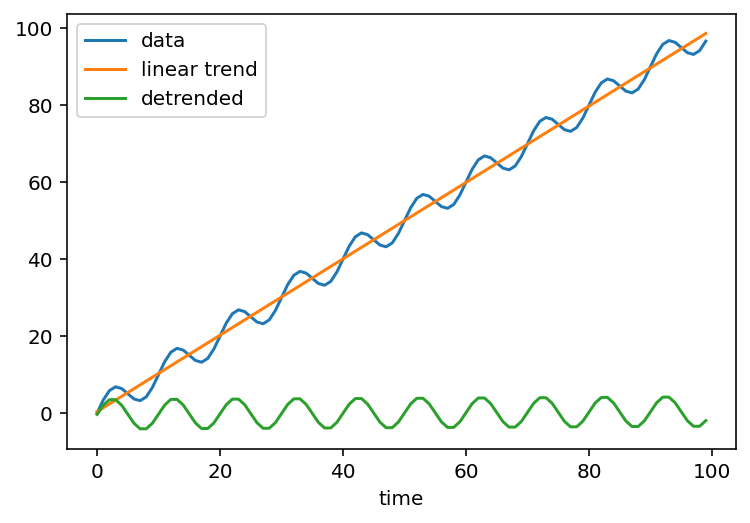
Here’s an example

Show code cell source Hide code cell source

import matplotlib.pyplot as plt
import numpy as np
import xarray as xr

time = np.arange(100)
data = time + 4 * np.sin(2 * np.pi / 10 * time)
da = xr.DataArray(data, dims="time", coords={"time": time})

# fit a straight line along time
p = da.polyfit(dim="time", deg=1, skipna=False)
# evaluate the linear trend as a timeseries
fit = xr.polyval(da["time"], p.polyfit_coefficients)


da.plot(label="data")
fit.plot(label="linear trend")
(da - fit).plot(label="detrended")
plt.legend()

<matplotlib.legend.Legend at 0x7fd46e54acd0>

Detrending with dask is a consistent source of headaches:

1. Polyfit performance on large datasets - Suboptimal dask task graph

2. Unexpected chunking of 3d DataArray in polyfit()

3. Memory errors with detrending + rolling operations

Challenges of detrending

Detrending has 3 steps:

1. Fit a polynomial using polyfit

2. Evaluate the trend using polyval and the fit coefficients

3. Subtract the trend from the original data

def detrend_dim(da, dim, deg=1):
    # detrend along a single dimension
    p = da.polyfit(dim=dim, deg=deg, skipna=False)
    fit = xr.polyval(da[dim], p.polyfit_coefficients)
    return da - fit

We usually want to subtract a linear trend in time. The main challenge is that model output is usually chunked with small chunksizes in time, and big chunksizes in space. Naively calling polyfit along time using xarray.apply_ufunc(numpy.polyfit, ..., dask="parallelized") would a require rechunking the dataset. This could be a good way to proceed if there are other time-series analyses that will be performed. In that case use rechunker.

DataArray.polyfit does actually support fitting along chunked dimensions. It uses dask.array.linalg.lstsq for an out-of-core parallel fitting algorithm.

However the limitation of lstsq is that it requires 2D arrays as input, but our model output is commonly 3D or 4D (time, depth, latitude, longitude). polyfit uses DataArray.stack to reshape all arrays to 2D, does the fit, and reshapes back. Easy, no?

Turns out… not easy. Reshaping in parallel can be really expensive! The dask docs illustrate this well. We have a possible solution but this hasn’t been implemented yet. It also turned out that this wasn’t the issue that affected Memory errors with detrending + rolling operations.

In this notebook, I explore the detrending problem a little bit to find what other challenges affect detrending workflows.

Summary

1. We use simple techniques like tracking chunk sizes and number of tasks to isolate a few problems, particularly in polyval.

2. Fixing polyval doesn’t improve the calculation, so we then examine the dask graph for polyfit in a smaller artificial problem that replicates the main issues.

3. This lets us trace the issue back to a serious regression in dask’s tensordot function.

4. That issue has since been fixed (available in dask >= 2022.03.0).

5. Now things work well!

Note

The first half of this notebook was built with dask==2021.12.0.

Setup

import dask.array
import distributed
import numpy as np
import xarray as xr
from IPython.display import Image

client = distributed.Client()
client

Client

Client-da6eb586-ab59-11ec-8493-3af9d394f1c6

Connection method: Cluster object	Cluster type: distributed.LocalCluster
Dashboard: http://127.0.0.1:8787/status

Cluster Info

LocalCluster

8e4cb217

Dashboard: http://127.0.0.1:8787/status	Workers: 4
Total threads: 8	Total memory: 16.00 GiB
Status: running	Using processes: True

Scheduler Info

Scheduler

Scheduler-adcbb9db-b9e8-46d6-a45a-67c8ba06d7e1

Comm: tcp://127.0.0.1:61123	Workers: 4
Dashboard: http://127.0.0.1:8787/status	Total threads: 8
Started: Just now	Total memory: 16.00 GiB

Workers

Worker: 0

Comm: tcp://127.0.0.1:61187	Total threads: 2
Dashboard: http://127.0.0.1:61191/status	Memory: 4.00 GiB
Nanny: tcp://127.0.0.1:61129
Local directory: /Users/dcherian/work/esds/blog/posts/2022/dask-worker-space/worker-7r12h0e2

Worker: 1

Comm: tcp://127.0.0.1:61188	Total threads: 2
Dashboard: http://127.0.0.1:61194/status	Memory: 4.00 GiB
Nanny: tcp://127.0.0.1:61132
Local directory: /Users/dcherian/work/esds/blog/posts/2022/dask-worker-space/worker-p3jqok8h

Worker: 2

Comm: tcp://127.0.0.1:61190	Total threads: 2
Dashboard: http://127.0.0.1:61192/status	Memory: 4.00 GiB
Nanny: tcp://127.0.0.1:61131
Local directory: /Users/dcherian/work/esds/blog/posts/2022/dask-worker-space/worker-1nc79fcf

Worker: 3

Comm: tcp://127.0.0.1:61189	Total threads: 2
Dashboard: http://127.0.0.1:61193/status	Memory: 4.00 GiB
Nanny: tcp://127.0.0.1:61130
Local directory: /Users/dcherian/work/esds/blog/posts/2022/dask-worker-space/worker-mq0h46t1

Example detrending operation

I’ll use the example dataset in Memory errors with detrending + rolling operations but make it smaller in time.

nt = 8772 // 4
ny = 489
nx = 655
# chunks like the data is stored on disk
# small in time, big in space
# because the chunk sizes are -1 along lat, lon;
# reshaping this array to (time, lat, lon) prior to fitting is pretty cheap
chunks = (8, -1, -1)

da = xr.DataArray(
    dask.array.random.random((nt, ny, nx), chunks=chunks),
    dims=("ocean_time", "eta_rho", "xi_rho"),
)
da

<xarray.DataArray 'random_sample-ffbb27b2e849e89719a8455875172787' (
                                                                    ocean_time: 2193,
                                                                    eta_rho: 489,
                                                                    xi_rho: 655)>
dask.array<random_sample, shape=(2193, 489, 655), dtype=float64, chunksize=(8, 489, 655), chunktype=numpy.ndarray>
Dimensions without coordinates: ocean_time, eta_rho, xi_rho

xarray.DataArray

'random_sample-ffbb27b2e849e89719a8455875172787'

• ocean_time: 2193
• eta_rho: 489
• xi_rho: 655

• dask.array<chunksize=(8, 489, 655), meta=np.ndarray>

  Array Chunk Bytes 5.23 GiB 19.55 MiB Shape (2193, 489, 655) (8, 489, 655) Count 275 Tasks 275 Chunks Type float64 numpy.ndarray

• Coordinates: (0)
• Attributes: (0)

# Function to detrend
# Source: https://gist.github.com/rabernat/1ea82bb067c3273a6166d1b1f77d490f


def detrend_dim(da, dim, deg=1):
    """detrend along a single dimension."""
    # calculate polynomial coefficients
    p = da.polyfit(dim=dim, deg=deg, skipna=False)
    # evaluate trend
    fit = xr.polyval(da[dim], p.polyfit_coefficients)
    # remove the trend
    return da - fit


detrended = detrend_dim(da, dim="ocean_time")
detrended

<xarray.DataArray (ocean_time: 2193, eta_rho: 489, xi_rho: 655)>
dask.array<sub, shape=(2193, 489, 655), dtype=float64, chunksize=(8, 489, 655), chunktype=numpy.ndarray>
Coordinates:
  * ocean_time  (ocean_time) int64 0 1 2 3 4 5 ... 2187 2188 2189 2190 2191 2192
  * eta_rho     (eta_rho) int64 0 1 2 3 4 5 6 7 ... 482 483 484 485 486 487 488
  * xi_rho      (xi_rho) int64 0 1 2 3 4 5 6 7 ... 648 649 650 651 652 653 654

xarray.DataArray

• ocean_time: 2193
• eta_rho: 489
• xi_rho: 655

• dask.array<chunksize=(8, 489, 655), meta=np.ndarray>

  Array Chunk Bytes 5.23 GiB 19.55 MiB Shape (2193, 489, 655) (8, 489, 655) Count 4803 Tasks 275 Chunks Type float64 numpy.ndarray

• Coordinates: (3)
  • ocean_time
    (ocean_time)
    int64
    0 1 2 3 4 ... 2189 2190 2191 2192

    array([   0,    1,    2, ..., 2190, 2191, 2192])

  • eta_rho
    (eta_rho)
    int64
    0 1 2 3 4 5 ... 484 485 486 487 488

    array([  0,   1,   2, ..., 486, 487, 488])

  • xi_rho
    (xi_rho)
    int64
    0 1 2 3 4 5 ... 650 651 652 653 654

    array([  0,   1,   2, ..., 652, 653, 654])

• Attributes: (0)

Warning

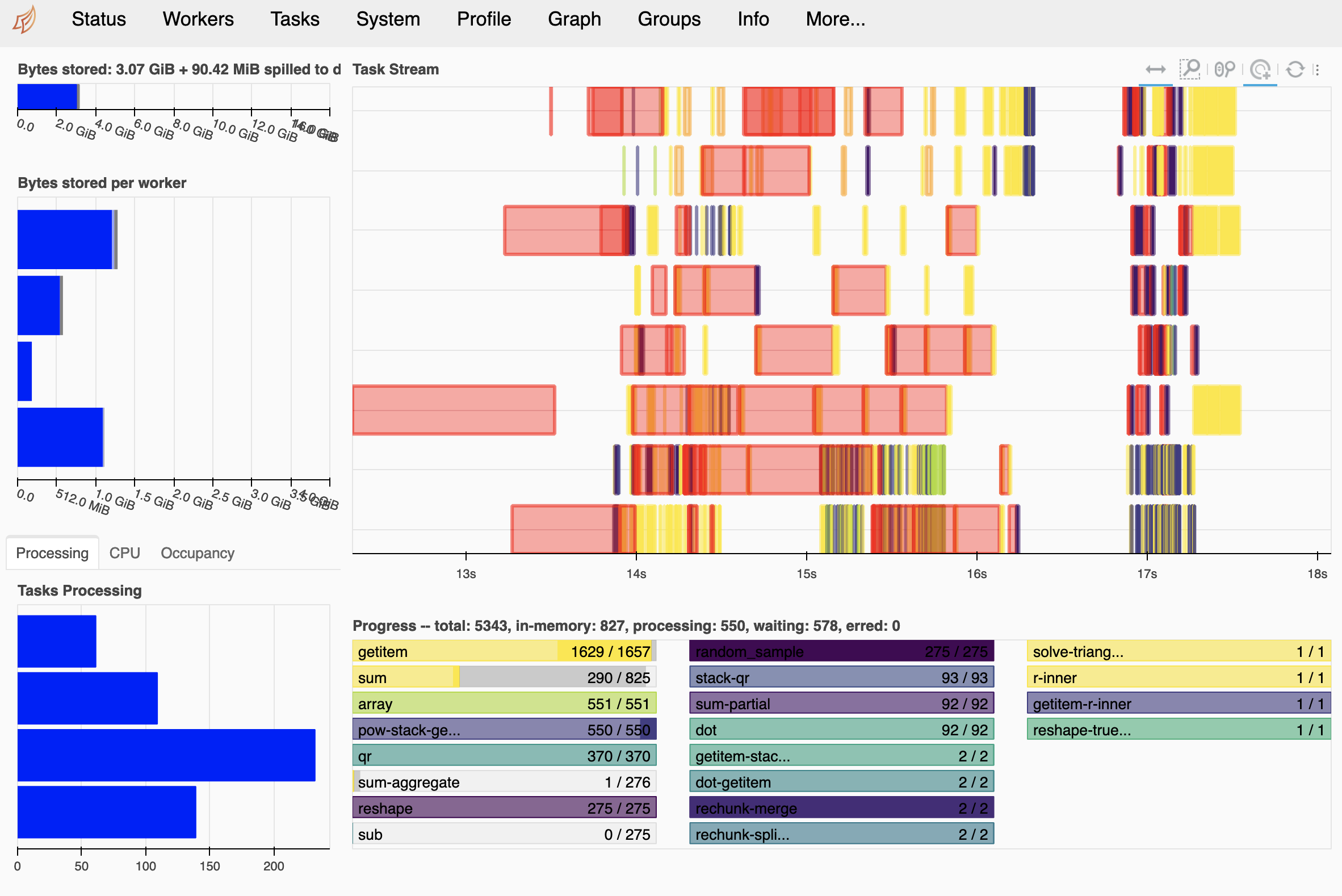
The dask dashboard screenshot for the following cell was captured with dask 2021.12.0.

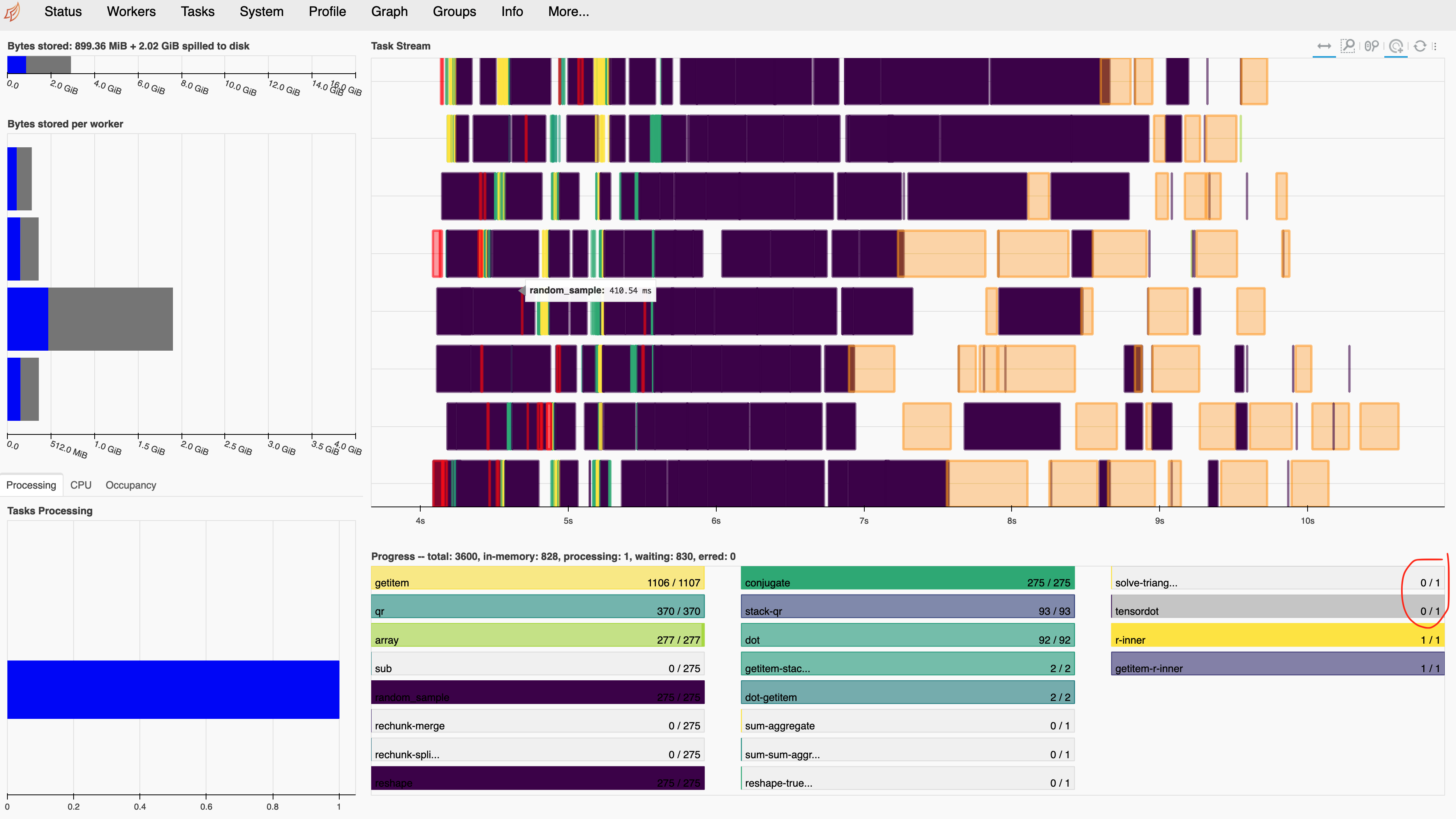
detrended.compute()

Calling compute doesn’t work so well and that single tensordot task looks funny. We have many input chunks and many output chunks. It’s not good if there’s a single task that might be a bottleneck by accumulating many input chunks.

Show code cell source Hide code cell source

Image("../images/detrend-dask-dashboard-1.png")

What is going wrong?

Lets look at detrend

Detrend has 3 steps:

1. polyfit

2. polyval

3. subtract

def detrend_dim(da, dim, deg=1):
    # detrend along a single dimension
    p = da.polyfit(dim=dim, deg=deg, skipna=False)
    fit = xr.polyval(da[dim], p.polyfit_coefficients)
    return da - fit

First lets try just polyfit.

# these are arguments provided to detrend
dim = "ocean_time"
deg = 1

p = da.polyfit(dim=dim, deg=deg, skipna=False)
p

<xarray.Dataset>
Dimensions:               (eta_rho: 489, xi_rho: 655, degree: 2)
Coordinates:
  * eta_rho               (eta_rho) int64 0 1 2 3 4 5 ... 484 485 486 487 488
  * xi_rho                (xi_rho) int64 0 1 2 3 4 5 ... 649 650 651 652 653 654
  * degree                (degree) int64 1 0
Data variables:
    polyfit_coefficients  (degree, eta_rho, xi_rho) float64 dask.array<chunksize=(2, 489, 655), meta=np.ndarray>

xarray.Dataset

• Dimensions:
  • eta_rho: 489
  • xi_rho: 655
  • degree: 2
• Coordinates: (3)
  • eta_rho
    (eta_rho)
    int64
    0 1 2 3 4 5 ... 484 485 486 487 488

    array([  0,   1,   2, ..., 486, 487, 488])

  • xi_rho
    (xi_rho)
    int64
    0 1 2 3 4 5 ... 650 651 652 653 654

    array([  0,   1,   2, ..., 652, 653, 654])

  • degree
    (degree)
    int64
    1 0

    array([1, 0])

• Data variables: (1)
  • polyfit_coefficients
    (degree, eta_rho, xi_rho)
    float64
    dask.array<chunksize=(2, 489, 655), meta=np.ndarray>

    Array Chunk Bytes 4.89 MiB 4.89 MiB Shape (2, 489, 655) (2, 489, 655) Count 3971 Tasks 1 Chunks Type float64 numpy.ndarray

• Attributes: (0)

Seems OK, by which I mean input chunks == output chunks.

How about polyval?

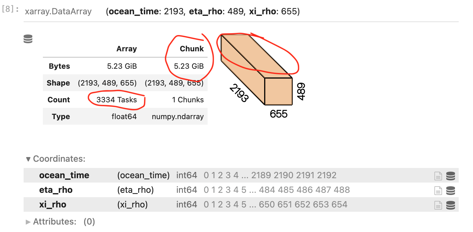
fit = xr.polyval(da[dim], p.polyfit_coefficients)
fit

<xarray.DataArray (ocean_time: 2193, eta_rho: 489, xi_rho: 655)>
dask.array<sum-aggregate, shape=(2193, 489, 655), dtype=float64, chunksize=(2193, 489, 655), chunktype=numpy.ndarray>
Coordinates:
  * ocean_time  (ocean_time) int64 0 1 2 3 4 5 ... 2187 2188 2189 2190 2191 2192
  * eta_rho     (eta_rho) int64 0 1 2 3 4 5 6 7 ... 482 483 484 485 486 487 488
  * xi_rho      (xi_rho) int64 0 1 2 3 4 5 6 7 ... 648 649 650 651 652 653 654

xarray.DataArray

• ocean_time: 2193
• eta_rho: 489
• xi_rho: 655

• dask.array<chunksize=(2193, 489, 655), meta=np.ndarray>

  Array Chunk Bytes 5.23 GiB 5.23 GiB Shape (2193, 489, 655) (2193, 489, 655) Count 3978 Tasks 1 Chunks Type float64 numpy.ndarray

• Coordinates: (3)
  • ocean_time
    (ocean_time)
    int64
    0 1 2 3 4 ... 2189 2190 2191 2192

    array([   0,    1,    2, ..., 2190, 2191, 2192])

  • eta_rho
    (eta_rho)
    int64
    0 1 2 3 4 5 ... 484 485 486 487 488

    array([  0,   1,   2, ..., 486, 487, 488])

  • xi_rho
    (xi_rho)
    int64
    0 1 2 3 4 5 ... 650 651 652 653 654

    array([  0,   1,   2, ..., 652, 653, 654])

• Attributes: (0)

Aha! Now suddenly we have one giant chunk for the entire array!

Show code cell source Hide code cell source

Image("../images/dask-repr.png")

Tip

The first step to checking your dask workflow is to look for sudden and large changes in number of tasks or chunk size. Pay attention to the dask repr.

Building a better polyval

To do this, we need to look closely at the code of polyval.

def polyval(coord, coeffs, degree_dim="degree"):
    from .dataarray import DataArray
    from .missing import get_clean_interp_index


    x = get_clean_interp_index(coord, coord.name, strict=False)


    deg_coord = coeffs[degree_dim]


    lhs = DataArray(
        np.vander(x, int(deg_coord.max()) + 1),
        dims=(coord.name, degree_dim),
        coords={coord.name: coord, degree_dim: np.arange(deg_coord.max() + 1)[::-1]},
    )
    return (lhs * coeffs).sum(degree_dim)

We call this using

    fit = xr.polyval(da[dim], p.polyfit_coefficients)

The core issue is that the da[dim] coord is unchunked. So lhs is a numpy array, which when combined with the coeffs (dask array) gives us a dask array with a single 5GB chunk.

da[dim]

<xarray.DataArray 'ocean_time' (ocean_time: 2193)>
array([   0,    1,    2, ..., 2190, 2191, 2192])
Dimensions without coordinates: ocean_time

xarray.DataArray

'ocean_time'

• ocean_time: 2193

• 0 1 2 3 4 5 6 7 8 9 ... 2184 2185 2186 2187 2188 2189 2190 2191 2192

  array([   0,    1,    2, ..., 2190, 2191, 2192])

• Coordinates: (0)
• Attributes: (0)

Let’s instead create a chunked “ocean_time” coordinate. This is a little roundabout because Xarray doesn’t let you chunk dimension coordinates using .chunk.

# first create a chunked version of the "ocean_time" dimension
chunked_dim = xr.DataArray(
    dask.array.from_array(da[dim].data, chunks=da.chunksizes[dim]), dims=dim, name=dim
)
chunked_dim

<xarray.DataArray 'ocean_time' (ocean_time: 2193)>
dask.array<array, shape=(2193,), dtype=int64, chunksize=(8,), chunktype=numpy.ndarray>
Dimensions without coordinates: ocean_time

xarray.DataArray

'ocean_time'

• ocean_time: 2193

• dask.array<chunksize=(8,), meta=np.ndarray>

  Array Chunk Bytes 17.13 kiB 64 B Shape (2193,) (8,) Count 275 Tasks 275 Chunks Type int64 numpy.ndarray

• Coordinates: (0)
• Attributes: (0)

This little bit is a rewritten version of polyval that can handle a chunked coord as input.

Note

This function will not work properly for an actual time coordinate. Here ocean_time is just ints. If it were a datetime vector, we would need to convert that to a vector of floats or ints.

def polyval(coord, coeffs, degree_dim="degree"):
    x = coord.data

    deg_coord = coeffs[degree_dim]
    N = int(deg_coord.max()) + 1

    lhs = xr.DataArray(
        np.stack([x ** (N - 1 - i) for i in range(N)], axis=1),
        dims=(coord.name, degree_dim),
        coords={coord.name: coord, degree_dim: np.arange(deg_coord.max() + 1)[::-1]},
    )
    return (lhs * coeffs).sum(degree_dim)


fit = polyval(chunked_dim, p.polyfit_coefficients)
fit

<xarray.DataArray (ocean_time: 2193, eta_rho: 489, xi_rho: 655)>
dask.array<sum-aggregate, shape=(2193, 489, 655), dtype=float64, chunksize=(8, 489, 655), chunktype=numpy.ndarray>
Coordinates:
  * ocean_time  (ocean_time) int64 0 1 2 3 4 5 ... 2187 2188 2189 2190 2191 2192
  * eta_rho     (eta_rho) int64 0 1 2 3 4 5 6 7 ... 482 483 484 485 486 487 488
  * xi_rho      (xi_rho) int64 0 1 2 3 4 5 6 7 ... 648 649 650 651 652 653 654

xarray.DataArray

• ocean_time: 2193
• eta_rho: 489
• xi_rho: 655

• dask.array<chunksize=(8, 489, 655), meta=np.ndarray>

  Array Chunk Bytes 5.23 GiB 19.55 MiB Shape (2193, 489, 655) (8, 489, 655) Count 8926 Tasks 275 Chunks Type float64 numpy.ndarray

• Coordinates: (3)
  • ocean_time
    (ocean_time)
    int64
    0 1 2 3 4 ... 2189 2190 2191 2192

    array([   0,    1,    2, ..., 2190, 2191, 2192])

  • eta_rho
    (eta_rho)
    int64
    0 1 2 3 4 5 ... 484 485 486 487 488

    array([  0,   1,   2, ..., 486, 487, 488])

  • xi_rho
    (xi_rho)
    int64
    0 1 2 3 4 5 ... 650 651 652 653 654

    array([  0,   1,   2, ..., 652, 653, 654])

• Attributes: (0)

An older dask version

Warning

The following cells describe an issue present for dask>2.30.0 and dask < 2022.03.0.

This is a much better fit but we still have issues computing it.

fit.compute()

Show code cell source Hide code cell source

Image("../images/detrend-dask-dashboard-2.png")

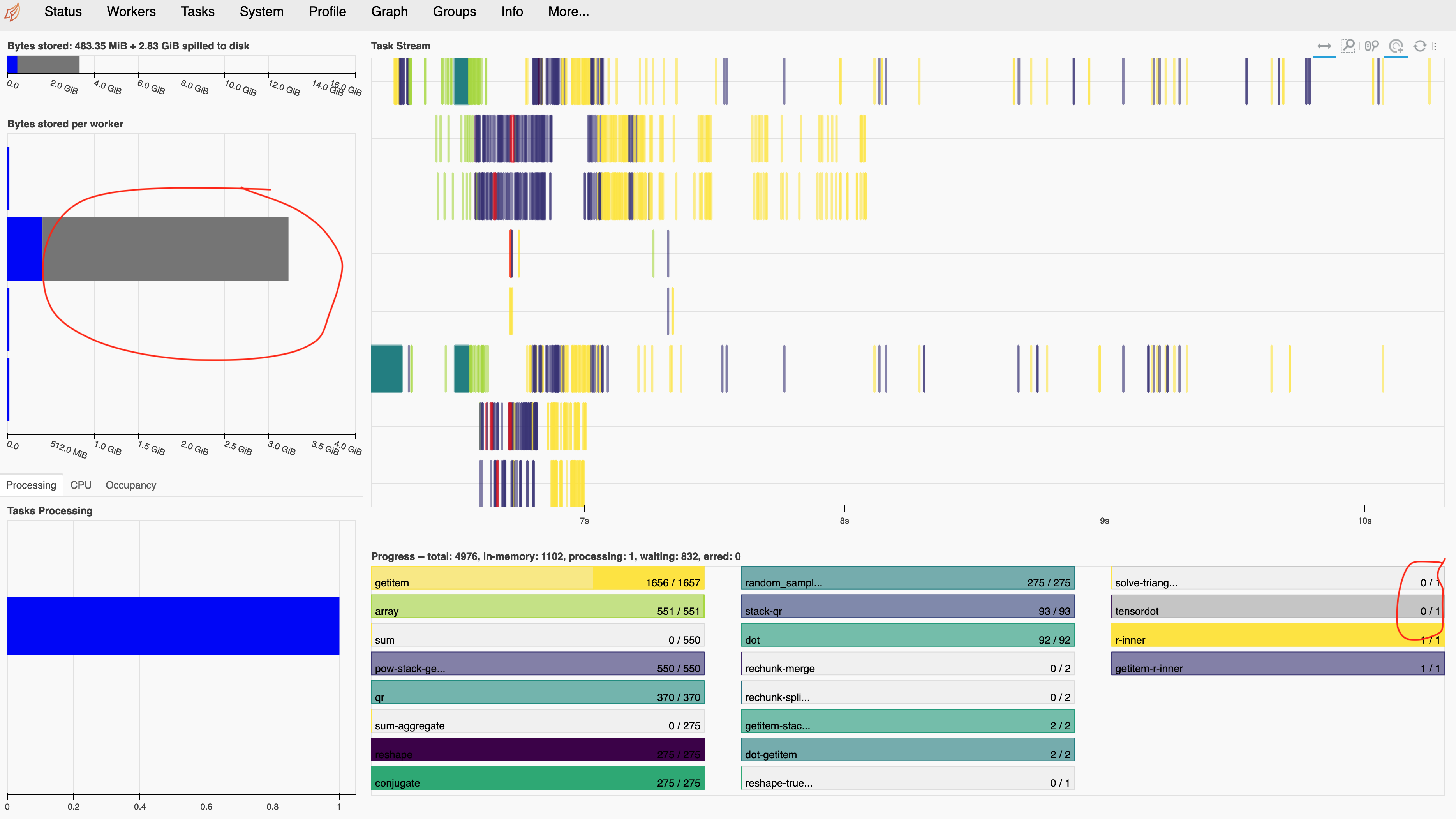
Hmm…. that single tensordot task still looks problematic. It is probably why we see very skewed memory consumption (mostly one worker).

Sadly and surprisingly, that wasn’t fixed by our new polyval!

Let’s look at polyfit again

A dask bug

But now for a much smaller problem.

Tip

Visualizing the dask graph can sometimes be instructive but really only works for small problems. Usually we want to see long parallel chains.

nt = 24
ny = 489
nx = 655
chunks = (8, -1, -1)

smol_da = xr.DataArray(
    dask.array.random.random((nt, ny, nx), chunks=chunks),
    dims=("ocean_time", "eta_rho", "xi_rho"),
)
smol_da

<xarray.DataArray 'random_sample-267f8112b7b54af2dbd898356bfcb6f7' (
                                                                    ocean_time: 24,
                                                                    eta_rho: 489,
                                                                    xi_rho: 655)>
dask.array<random_sample, shape=(24, 489, 655), dtype=float64, chunksize=(8, 489, 655), chunktype=numpy.ndarray>
Dimensions without coordinates: ocean_time, eta_rho, xi_rho

xarray.DataArray

'random_sample-267f8112b7b54af2dbd898356bfcb6f7'

• ocean_time: 24
• eta_rho: 489
• xi_rho: 655

• dask.array<chunksize=(8, 489, 655), meta=np.ndarray>

  Array Chunk Bytes 58.65 MiB 19.55 MiB Shape (24, 489, 655) (8, 489, 655) Count 3 Tasks 3 Chunks Type float64 numpy.ndarray

• Coordinates: (0)
• Attributes: (0)

p = smol_da.polyfit(dim="ocean_time", deg=1, skipna=False)
dask.visualize(p, rankdir="LR")

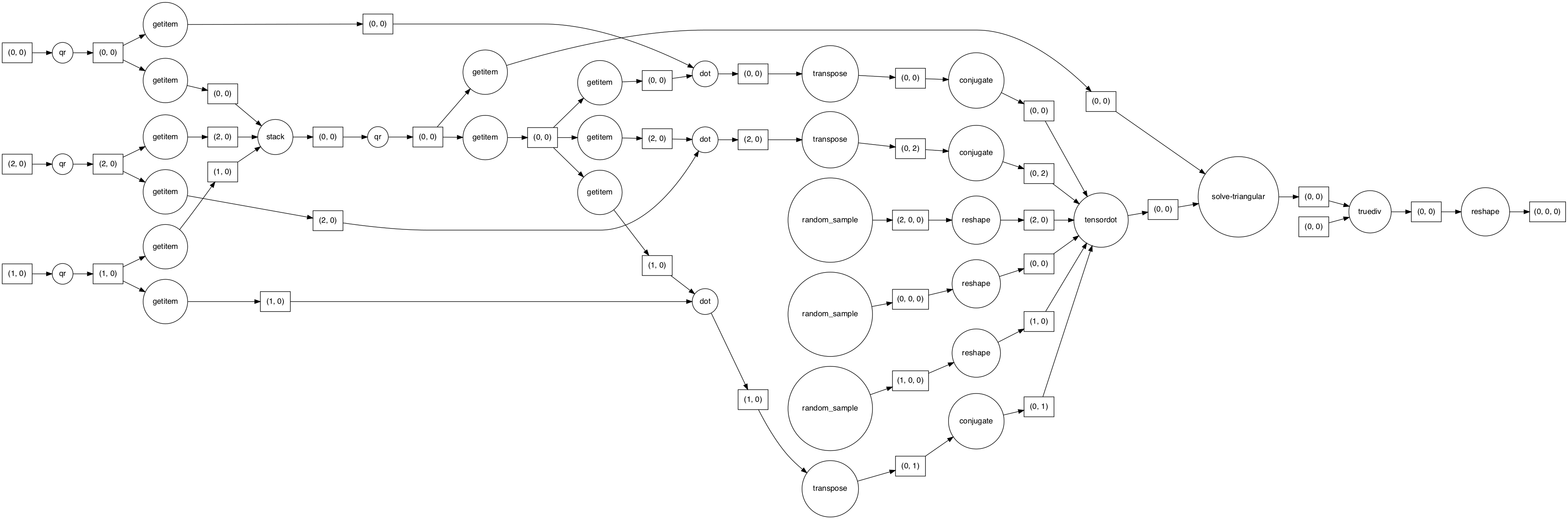
Ouch. we see all the tasks go through a single tensordot task.

This cannot work well. It effectively means that one worker is going to receive all time steps as a single chunk, which implies a lot of memory use and network transfer.

Searching the dask issue tracker leads to this issue so we were stuck.

Is it fixed?

Thanks to some upstream work in dask, we expect the tensordot problem is fixed. So let’s try it again.

Upgrading dask to dask==2022.03.0 shows a much better graph.

dask.__version__

'2022.03.0'

p = smol_da.polyfit(dim="ocean_time", deg=1, skipna=False)
dask.visualize(p, rankdir="LR")

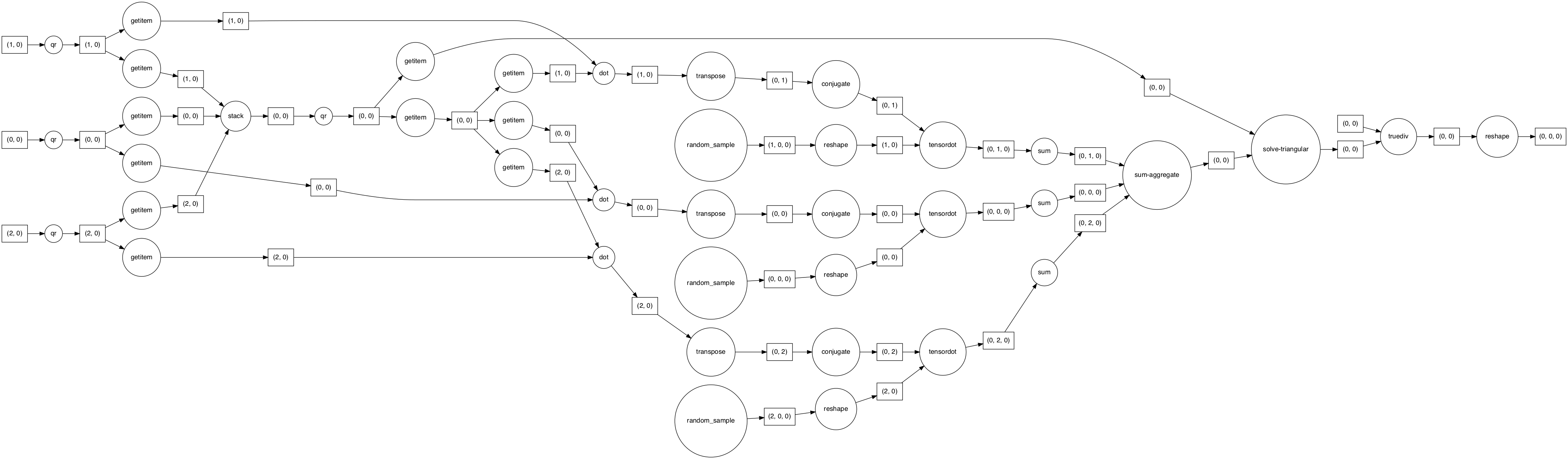
Yes! we now see 3 tensordot tasks for this smaller problem instead of 1 in the previous buggy version.

Attempt 2

# these are arguments provided to detrend
dim = "ocean_time"
deg = 1

p = da.polyfit(dim=dim, deg=deg, skipna=False)
p

<xarray.Dataset>
Dimensions:               (eta_rho: 489, xi_rho: 655, degree: 2)
Coordinates:
  * eta_rho               (eta_rho) int64 0 1 2 3 4 5 ... 484 485 486 487 488
  * xi_rho                (xi_rho) int64 0 1 2 3 4 5 ... 649 650 651 652 653 654
  * degree                (degree) int64 1 0
Data variables:
    polyfit_coefficients  (degree, eta_rho, xi_rho) float64 dask.array<chunksize=(2, 489, 655), meta=np.ndarray>

xarray.Dataset

• Dimensions:
  • eta_rho: 489
  • xi_rho: 655
  • degree: 2
• Coordinates: (3)
  • eta_rho
    (eta_rho)
    int64
    0 1 2 3 4 5 ... 484 485 486 487 488

    array([  0,   1,   2, ..., 486, 487, 488])

  • xi_rho
    (xi_rho)
    int64
    0 1 2 3 4 5 ... 650 651 652 653 654

    array([  0,   1,   2, ..., 652, 653, 654])

  • degree
    (degree)
    int64
    1 0

    array([1, 0])

• Data variables: (1)
  • polyfit_coefficients
    (degree, eta_rho, xi_rho)
    float64
    dask.array<chunksize=(2, 489, 655), meta=np.ndarray>

    Array Chunk Bytes 4.89 MiB 4.89 MiB Shape (2, 489, 655) (2, 489, 655) Count 3971 Tasks 1 Chunks Type float64 numpy.ndarray

• Attributes: (0)

Computing works very well.

p.compute()

<xarray.Dataset>
Dimensions:               (eta_rho: 489, xi_rho: 655, degree: 2)
Coordinates:
  * eta_rho               (eta_rho) int64 0 1 2 3 4 5 ... 484 485 486 487 488
  * xi_rho                (xi_rho) int64 0 1 2 3 4 5 ... 649 650 651 652 653 654
  * degree                (degree) int64 1 0
Data variables:
    polyfit_coefficients  (degree, eta_rho, xi_rho) float64 1.756e-06 ... 0.5212

xarray.Dataset

• Dimensions:
  • eta_rho: 489
  • xi_rho: 655
  • degree: 2
• Coordinates: (3)
  • eta_rho
    (eta_rho)
    int64
    0 1 2 3 4 5 ... 484 485 486 487 488

    array([  0,   1,   2, ..., 486, 487, 488])

  • xi_rho
    (xi_rho)
    int64
    0 1 2 3 4 5 ... 650 651 652 653 654

    array([  0,   1,   2, ..., 652, 653, 654])

  • degree
    (degree)
    int64
    1 0

    array([1, 0])

• Data variables: (1)
  • polyfit_coefficients
    (degree, eta_rho, xi_rho)
    float64
    1.756e-06 -7.615e-06 ... 0.5212

    array([[[ 1.75581496e-06, -7.61467574e-06, -2.44002406e-06, ...,
              1.12309913e-05, -1.44585338e-05,  2.56390013e-06],
            [ 6.24806791e-06, -6.15844975e-06, -3.47201141e-06, ...,
             -3.02758525e-06,  9.28901640e-06, -4.35247403e-06],
            [ 3.14059230e-06, -2.73902120e-06,  4.36798033e-06, ...,
              2.69570066e-06,  1.21424802e-05, -1.19296261e-05],
            ...,
            [-1.39630478e-05, -4.30467797e-07,  4.49269076e-06, ...,
             -1.74598346e-06, -4.47517149e-06,  1.72432654e-06],
            [-1.80066936e-05, -7.42672688e-06,  6.37428615e-06, ...,
              2.25875887e-08,  4.47743868e-06, -6.17660861e-06],
            [ 7.84220832e-06,  2.33238192e-06, -4.15524177e-06, ...,
             -4.55852034e-06,  1.63251636e-05, -1.22139278e-05]],
    
           [[ 5.05756495e-01,  5.05097856e-01,  5.10282701e-01, ...,
              4.91170191e-01,  5.10311168e-01,  5.02607227e-01],
            [ 5.03647573e-01,  4.99178698e-01,  4.99817482e-01, ...,
              5.02750949e-01,  4.94620384e-01,  5.10763635e-01],
            [ 4.86849939e-01,  4.95366172e-01,  4.89458361e-01, ...,
              4.97706761e-01,  4.94095708e-01,  5.15752314e-01],
            ...,
            [ 5.03503042e-01,  4.99954669e-01,  4.87935564e-01, ...,
              4.96127947e-01,  5.05013439e-01,  4.99296571e-01],
            [ 5.26822889e-01,  5.00025932e-01,  5.00574897e-01, ...,
              4.95895063e-01,  4.99121132e-01,  4.97883158e-01],
            [ 5.00344152e-01,  5.03210576e-01,  4.96368482e-01, ...,
              4.96429148e-01,  4.73881900e-01,  5.21241603e-01]]])

• Attributes: (0)

fit = polyval(chunked_dim, p.polyfit_coefficients)
fit

<xarray.DataArray (ocean_time: 2193, eta_rho: 489, xi_rho: 655)>
dask.array<sum-aggregate, shape=(2193, 489, 655), dtype=float64, chunksize=(8, 489, 655), chunktype=numpy.ndarray>
Coordinates:
  * ocean_time  (ocean_time) int64 0 1 2 3 4 5 ... 2187 2188 2189 2190 2191 2192
  * eta_rho     (eta_rho) int64 0 1 2 3 4 5 6 7 ... 482 483 484 485 486 487 488
  * xi_rho      (xi_rho) int64 0 1 2 3 4 5 6 7 ... 648 649 650 651 652 653 654

xarray.DataArray

• ocean_time: 2193
• eta_rho: 489
• xi_rho: 655

• dask.array<chunksize=(8, 489, 655), meta=np.ndarray>

  Array Chunk Bytes 5.23 GiB 19.55 MiB Shape (2193, 489, 655) (8, 489, 655) Count 8926 Tasks 275 Chunks Type float64 numpy.ndarray

• Coordinates: (3)
  • ocean_time
    (ocean_time)
    int64
    0 1 2 3 4 ... 2189 2190 2191 2192

    array([   0,    1,    2, ..., 2190, 2191, 2192])

  • eta_rho
    (eta_rho)
    int64
    0 1 2 3 4 5 ... 484 485 486 487 488

    array([  0,   1,   2, ..., 486, 487, 488])

  • xi_rho
    (xi_rho)
    int64
    0 1 2 3 4 5 ... 650 651 652 653 654

    array([  0,   1,   2, ..., 652, 653, 654])

• Attributes: (0)

fit.compute()

<xarray.DataArray (ocean_time: 2193, eta_rho: 489, xi_rho: 655)>
array([[[0.5057565 , 0.50509786, 0.5102827 , ..., 0.49117019,
         0.51031117, 0.50260723],
        [0.50364757, 0.4991787 , 0.49981748, ..., 0.50275095,
         0.49462038, 0.51076364],
        [0.48684994, 0.49536617, 0.48945836, ..., 0.49770676,
         0.49409571, 0.51575231],
        ...,
        [0.50350304, 0.49995467, 0.48793556, ..., 0.49612795,
         0.50501344, 0.49929657],
        [0.52682289, 0.50002593, 0.5005749 , ..., 0.49589506,
         0.49912113, 0.49788316],
        [0.50034415, 0.50321058, 0.49636848, ..., 0.49642915,
         0.4738819 , 0.5212416 ]],

       [[0.50575825, 0.50509024, 0.51028026, ..., 0.49118142,
         0.51029671, 0.50260979],
        [0.50365382, 0.49917254, 0.49981401, ..., 0.50274792,
         0.49462967, 0.51075928],
        [0.48685308, 0.49536343, 0.48946273, ..., 0.49770946,
         0.49410785, 0.51574038],
...
        [0.47291   , 0.49901151, 0.49777905, ..., 0.4923025 ,
         0.49520834, 0.50307457],
        [0.48737022, 0.48375397, 0.51454096, ..., 0.49594455,
         0.5089312 , 0.48435021],
        [0.51752643, 0.50832082, 0.48726435, ..., 0.48644143,
         0.50965033, 0.49448089]],

       [[0.50960524, 0.48840649, 0.50493417, ..., 0.51578852,
         0.47861806, 0.5082273 ],
        [0.51734334, 0.48567938, 0.49220683, ..., 0.49611448,
         0.51498191, 0.50122301],
        [0.49373412, 0.48936224, 0.49903297, ..., 0.50361574,
         0.52071202, 0.48960257],
        ...,
        [0.47289604, 0.49901108, 0.49778354, ..., 0.49230075,
         0.49520386, 0.50307629],
        [0.48735222, 0.48374655, 0.51454733, ..., 0.49594458,
         0.50893568, 0.48434403],
        [0.51753427, 0.50832316, 0.48726019, ..., 0.48643687,
         0.50966666, 0.49446867]]])
Coordinates:
  * ocean_time  (ocean_time) int64 0 1 2 3 4 5 ... 2187 2188 2189 2190 2191 2192
  * eta_rho     (eta_rho) int64 0 1 2 3 4 5 6 7 ... 482 483 484 485 486 487 488
  * xi_rho      (xi_rho) int64 0 1 2 3 4 5 6 7 ... 648 649 650 651 652 653 654

xarray.DataArray

• ocean_time: 2193
• eta_rho: 489
• xi_rho: 655

• 0.5058 0.5051 0.5103 0.5048 0.5073 ... 0.5073 0.4864 0.5097 0.4945

  array([[[0.5057565 , 0.50509786, 0.5102827 , ..., 0.49117019,
           0.51031117, 0.50260723],
          [0.50364757, 0.4991787 , 0.49981748, ..., 0.50275095,
           0.49462038, 0.51076364],
          [0.48684994, 0.49536617, 0.48945836, ..., 0.49770676,
           0.49409571, 0.51575231],
          ...,
          [0.50350304, 0.49995467, 0.48793556, ..., 0.49612795,
           0.50501344, 0.49929657],
          [0.52682289, 0.50002593, 0.5005749 , ..., 0.49589506,
           0.49912113, 0.49788316],
          [0.50034415, 0.50321058, 0.49636848, ..., 0.49642915,
           0.4738819 , 0.5212416 ]],
  
         [[0.50575825, 0.50509024, 0.51028026, ..., 0.49118142,
           0.51029671, 0.50260979],
          [0.50365382, 0.49917254, 0.49981401, ..., 0.50274792,
           0.49462967, 0.51075928],
          [0.48685308, 0.49536343, 0.48946273, ..., 0.49770946,
           0.49410785, 0.51574038],
  ...
          [0.47291   , 0.49901151, 0.49777905, ..., 0.4923025 ,
           0.49520834, 0.50307457],
          [0.48737022, 0.48375397, 0.51454096, ..., 0.49594455,
           0.5089312 , 0.48435021],
          [0.51752643, 0.50832082, 0.48726435, ..., 0.48644143,
           0.50965033, 0.49448089]],
  
         [[0.50960524, 0.48840649, 0.50493417, ..., 0.51578852,
           0.47861806, 0.5082273 ],
          [0.51734334, 0.48567938, 0.49220683, ..., 0.49611448,
           0.51498191, 0.50122301],
          [0.49373412, 0.48936224, 0.49903297, ..., 0.50361574,
           0.52071202, 0.48960257],
          ...,
          [0.47289604, 0.49901108, 0.49778354, ..., 0.49230075,
           0.49520386, 0.50307629],
          [0.48735222, 0.48374655, 0.51454733, ..., 0.49594458,
           0.50893568, 0.48434403],
          [0.51753427, 0.50832316, 0.48726019, ..., 0.48643687,
           0.50966666, 0.49446867]]])

• Coordinates: (3)
  • ocean_time
    (ocean_time)
    int64
    0 1 2 3 4 ... 2189 2190 2191 2192

    array([   0,    1,    2, ..., 2190, 2191, 2192])

  • eta_rho
    (eta_rho)
    int64
    0 1 2 3 4 5 ... 484 485 486 487 488

    array([  0,   1,   2, ..., 486, 487, 488])

  • xi_rho
    (xi_rho)
    int64
    0 1 2 3 4 5 ... 650 651 652 653 654

    array([  0,   1,   2, ..., 652, 653, 654])

• Attributes: (0)

This ends up working well!

Show code cell source Hide code cell source

Image("../images/detrend-dask-dashboard-3.png")

Finally

Here’s everything put together:

def polyval(coord, coeffs, degree_dim="degree"):
    x = coord.data

    deg_coord = coeffs[degree_dim]
    N = int(deg_coord.max()) + 1

    lhs = xr.DataArray(
        np.stack([x ** (N - 1 - i) for i in range(N)], axis=1),
        dims=(coord.name, degree_dim),
        coords={coord.name: coord, degree_dim: np.arange(deg_coord.max() + 1)[::-1]},
    )
    return (lhs * coeffs).sum(degree_dim)


# Function to detrend
# Modified from source: https://gist.github.com/rabernat/1ea82bb067c3273a6166d1b1f77d490f
def detrend_dim(da, dim, deg=1):
    """detrend along a single dimension."""
    # calculate polynomial coefficients
    p = da.polyfit(dim=dim, deg=deg, skipna=False)
    # first create a chunked version of the "ocean_time" dimension
    chunked_dim = xr.DataArray(
        dask.array.from_array(da[dim].data, chunks=da.chunksizes[dim]),
        dims=dim,
        name=dim,
    )
    fit = polyval(chunked_dim, p.polyfit_coefficients)
    # evaluate trend
    # remove the trend
    return da - fit


detrended = detrend_dim(da, dim="ocean_time")
detrended

<xarray.DataArray (ocean_time: 2193, eta_rho: 489, xi_rho: 655)>
dask.array<sub, shape=(2193, 489, 655), dtype=float64, chunksize=(8, 489, 655), chunktype=numpy.ndarray>
Coordinates:
  * ocean_time  (ocean_time) int64 0 1 2 3 4 5 ... 2187 2188 2189 2190 2191 2192
  * eta_rho     (eta_rho) int64 0 1 2 3 4 5 6 7 ... 482 483 484 485 486 487 488
  * xi_rho      (xi_rho) int64 0 1 2 3 4 5 6 7 ... 648 649 650 651 652 653 654

xarray.DataArray

• ocean_time: 2193
• eta_rho: 489
• xi_rho: 655

• dask.array<chunksize=(8, 489, 655), meta=np.ndarray>

  Array Chunk Bytes 5.23 GiB 19.55 MiB Shape (2193, 489, 655) (8, 489, 655) Count 9201 Tasks 275 Chunks Type float64 numpy.ndarray

• Coordinates: (3)
  • ocean_time
    (ocean_time)
    int64
    0 1 2 3 4 ... 2189 2190 2191 2192

    array([   0,    1,    2, ..., 2190, 2191, 2192])

  • eta_rho
    (eta_rho)
    int64
    0 1 2 3 4 5 ... 484 485 486 487 488

    array([  0,   1,   2, ..., 486, 487, 488])

  • xi_rho
    (xi_rho)
    int64
    0 1 2 3 4 5 ... 650 651 652 653 654

    array([  0,   1,   2, ..., 652, 653, 654])

• Attributes: (0)

detrended.compute()

Show code cell source Hide code cell source

Image("../images/detrend-dask-dashboard-4.png")

It works!

Summary

In this notebook, I explore the detrending problem a little bit to find what other challenges affect detrending workflows.

1. We use simple techniques like tracking chunk sizes and number of tasks to isolate a few problems.

2. Fixing those doesn’t improve the calculation, so we then examine the dask graph for a smaller artificial problem that replicates the main issues.

3. This lets us trace the issue back to a serious regression in dask.

4. That issue has now been fixed.

5. And things work!

Future work

1. Some improvements to xarray.polyval are needed so that it can handle a chunked coordinate as input.

2. Dask could also detect that a giant 5GB chunk is constructed by this line in polyval:

   (lhs * coeffs).sum(degree_dim)
   

   and automatically avoid this problem by rechunking lhs prior to multiplying.

Batch Processing Jupyter Notebooks with Papermill   The Python Tutorial Series Returns this Summer!