Spectral Analysis#
This example demonstrates how to perform spectral and cross-spectral analysis.
This document shows a concise workflow using the scipy.signal module. To learn more about the functions and keyword arguments available in this package, read SciPy’s signal processing documentation.
This notebook will cover:
Periodograms
Smoothing
Cross Spectral Analysis
Coherence
import xarray as xr
import geocat.datafiles as gcd
import pandas as pd
import scipy
import matplotlib.pyplot as plt
import numpy as np
Periodogram#
A periodogram estimate is the square of the coefficients from the Fourier transform of one dimension of spectral data.
Read in Data#
We’ll use the geocat-datafiles module to access the relevant datafile for this example: SOI_Darwin.nc
Then, we use xarray.open_dataset() function to read the data as an xarray dataset.
This data represents the Darwin Southern Oscillation Index between 1882 and 1998 using normalized sea level pressure.
soi_darwin = xr.open_dataset(gcd.get('netcdf_files/SOI_Darwin.nc'))

soi_darwin
Downloading file 'netcdf_files/SOI_Darwin.nc' from 'https://github.com/NCAR/GeoCAT-datafiles/raw/main/netcdf_files/SOI_Darwin.nc' to '/home/runner/.cache/geocat'.
<xarray.Dataset> Size: 22kB
Dimensions:  (time: 1404)
Coordinates:
  * time     (time) int32 6kB 0 1 2 3 4 5 6 ... 1398 1399 1400 1401 1402 1403
Data variables:
    date     (time) float64 11kB ...
    DSOI     (time) float32 6kB ...
Attributes:
    title:          Darwin Southern Oscillation Index
    source:         Climate Analysis Section, NCAR
    history:        \nDSOI = - Normalized Darwin\nNormalized sea level pressu...
    creation_date:  Tue Mar 30 09:29:20 MST 1999
    references:     Trenberth, Mon. Wea. Rev: 2/1984
    time_span:      1882 - 1998
conventions: NoneTime Series Correction#
Currently, our time coordinate is in units of months since January 1882, we’ll use pandas to change this to the conventional DatetimeIndex.
start_date = pd.Timestamp('1882-01-01')
dates = [
    start_date + pd.DateOffset(months=int(month))
    for month in soi_darwin.indexes['time']
]
datetime_index = pd.DatetimeIndex(dates)

datetime_index
DatetimeIndex(['1882-01-01', '1882-02-01', '1882-03-01', '1882-04-01',
               '1882-05-01', '1882-06-01', '1882-07-01', '1882-08-01',
               '1882-09-01', '1882-10-01',
               ...
               '1998-03-01', '1998-04-01', '1998-05-01', '1998-06-01',
               '1998-07-01', '1998-08-01', '1998-09-01', '1998-10-01',
               '1998-11-01', '1998-12-01'],
              dtype='datetime64[ns]', length=1404, freq=None)
soi = soi_darwin.DSOI
soi['time'] = datetime_index
Periodogram#
Now we can call scipy.signal.periodogram().
You can specify a window argument for smoothing your spectrum before spectral analysis. Here is a list of supported Scipy windows. The default is boxcar which is a unit window equivalent to no tapering.
Set the detrending kwarg to constant to remove the mean from our data.
There is also a scaling keyword that defaults to density for computing the power spectral density with units of \(V^{2}/Hz\), with V being the units of the input array (here dimensionless), and Hz representing your frequency units (we’ll use per month instead of per second). spectral is also supported and produces the squared magnitude spectrum with units of \(V^{2}\).
freq_soi, psd_soi = scipy.signal.periodogram(
    soi,
    fs=1,  # sample monthly
    window='tukey',
    detrend='constant',
)
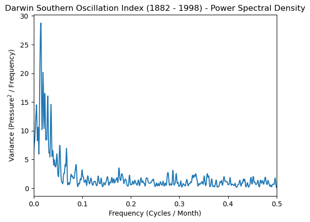
Smoothing#
To provide statistical reliability, the periodogram estimates must be smoothed.
You can use the same scipy.signal.windows as for the tapering. We’ll chose a standard Hann window.
k = 3  # smoothing constant

window = scipy.signal.windows.hann(2 * k + 1)  # Hann Window
window = window / window.sum()  # Normalize window

# Apply the convolution
smoothed_psd = scipy.signal.convolve(psd_soi, window, mode='same')
Plot#
plt.plot(freq_soi, smoothed_psd)
plt.xlabel('Frequency (Cycles / Month)')
plt.ylabel('Variance (Pressure$^2$ / Frequency)')
plt.title('Darwin Southern Oscillation Index (1882 - 1998) - Power Spectral Density')
plt.xlim([0, 0.5]);
Cross-Spectral Analysis#
For cross-spectral analysis, we’ll create plots of the following quantities: cospectrum, quadtrature, phase, coherence squared, and the periodogram of each dimensional array.
Read in Data#
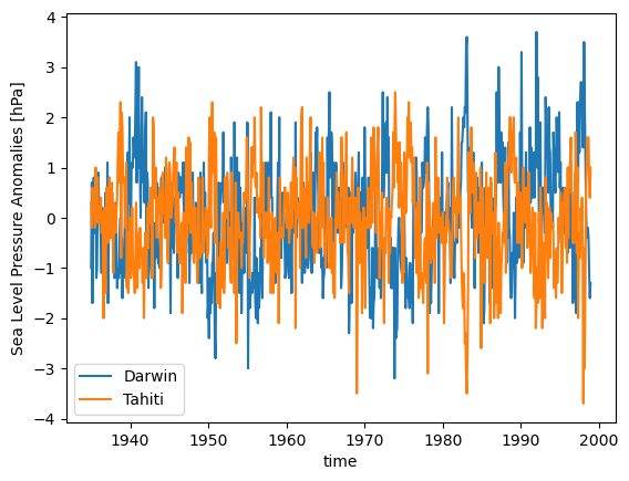
For our cross-spectral data we’ll look at SLP_DarwinTahitiAnom which contains Darwin and Tahiti sea level pressure anomalies between 1935-1998.
This data will need the same time series adjustment as in the periodogram example above.
slp_darwin = xr.open_dataset(gcd.get('netcdf_files/SLP_DarwinTahitiAnom.nc'))

# Time Series Correction
start_date = pd.Timestamp('1935-01-01')  # Months Since January 1935
dates = [
    start_date + pd.DateOffset(months=int(month))
    for month in slp_darwin.indexes['time']
]
datetime_index = pd.DatetimeIndex(dates)

slp_darwin['time'] = datetime_index
slp_darwin
Downloading file 'netcdf_files/SLP_DarwinTahitiAnom.nc' from 'https://github.com/NCAR/GeoCAT-datafiles/raw/main/netcdf_files/SLP_DarwinTahitiAnom.nc' to '/home/runner/.cache/geocat'.
<xarray.Dataset> Size: 18kB
Dimensions:  (time: 768)
Coordinates:
  * time     (time) datetime64[ns] 6kB 1935-01-01 1935-02-01 ... 1998-12-01
Data variables:
    date     (time) float64 6kB ...
    DSLP     (time) float32 3kB ...
    TSLP     (time) float32 3kB ...
Attributes:
    title:          Darwin and Tahiti Sea Level Pressure Anomalies: 1935-1998
    source:         Climate Analysis Section, NCAR
    history:        \nCreated to test specxy routines
    creation_date:  Tue Mar 30 12:34:39 MST 1999
conventions: Nonedslp = slp_darwin.DSLP # Darwin
dslp
<xarray.DataArray 'DSLP' (time: 768)> Size: 3kB
[768 values with dtype=float32]
Coordinates:
  * time     (time) datetime64[ns] 6kB 1935-01-01 1935-02-01 ... 1998-12-01
Attributes:
    short_name:  DSLP
    long_name:   Darwin Sea Level Pressure Anomalies
units: hPatslp = slp_darwin.TSLP # Tahiti
tslp
<xarray.DataArray 'TSLP' (time: 768)> Size: 3kB
[768 values with dtype=float32]
Coordinates:
  * time     (time) datetime64[ns] 6kB 1935-01-01 1935-02-01 ... 1998-12-01
Attributes:
    short_name:  TSLP
    long_name:   Tahiti Sea Level Pressure Anomalies
units: hPadslp.plot(label='Darwin')
tslp.plot(label='Tahiti')
plt.legend()
plt.ylabel('Sea Level Pressure Anomalies [hPa]');
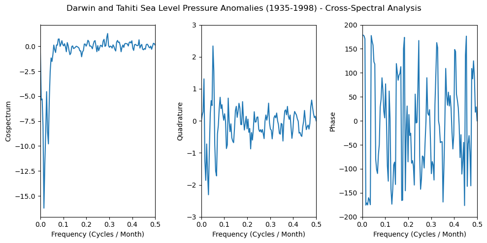
Cross-Power Spectral Density#
We will calculate cospectrum, quadtrature, and phase by leveraging scipy.signal.csd() and computing its real (cospectrum) and imaginary (quadtrature) components, and calculating the angle between them (phase).
f, pxy = scipy.signal.csd(
    dslp,
    tslp,
    fs=1,  # monthly
    detrend='constant',
)  # remove mean

cospectrum = np.real(pxy)
quadrature = np.imag(pxy)

phase = np.angle(pxy, deg=True)
fig, axs = plt.subplots(1, 3, figsize=(10, 5))

axs[0].plot(f, cospectrum)
axs[0].set_xlim([0, 0.5])
axs[0].set_xlabel('Frequency (Cycles / Month)')
axs[0].set_ylabel('Cospectrum')

axs[1].plot(f, quadrature)
axs[1].set_xlim([0, 0.5])
axs[1].set_ylim([-3, 3])
axs[1].set_xlabel('Frequency (Cycles / Month)')
axs[1].set_ylabel('Quadrature')

axs[2].plot(f, phase)
axs[2].set_xlim([0, 0.5])
axs[2].set_ylim([-200, 200])
axs[2].set_xlabel('Frequency (Cycles / Month)')
axs[2].set_ylabel('Phase')

fig.suptitle(
    'Darwin and Tahiti Sea Level Pressure Anomalies (1935-1998) - Cross-Spectral Analysis'
)
plt.tight_layout();
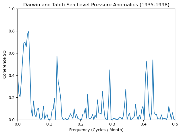
Coherence Squared#
Coherence is a measure of how similar two specta are, with regards to their frequency and phase offset relative to one another.
For coherence squared, simply square the output from scipy.signal.coherence().
f, cxy = scipy.signal.coherence(
    dslp,
    tslp,
    fs=1,  # monthly
    detrend='constant',
)  # remove mean

co_sq = cxy**2
plt.plot(f, co_sq)
plt.xlim([0, 0.5])
plt.ylim([0, 1])
plt.xlabel('Frequency (Cycles / Month)')
plt.ylabel('Coherence SQ')

plt.title('Darwin and Tahiti Sea Level Pressure Anomalies (1935-1998)')
plt.tight_layout();
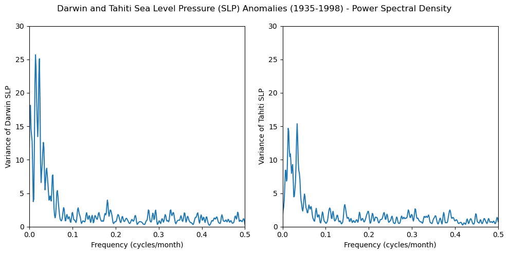
Peridogram and Smoothing#
# Calculate Periodogram
freq_dslp, dslp_psd = scipy.signal.periodogram(
    dslp,
    fs=1,  # monthly
    detrend='constant',
)  # remove mean
freq_tslp, tslp_psd = scipy.signal.periodogram(tslp, fs=1, detrend='constant')

# Perform modified Daniel Smoothing
dslp_smoothed = scipy.signal.convolve(dslp_psd, window, mode='same')
tslp_smoothed = scipy.signal.convolve(tslp_psd, window, mode='same')
fig, axs = plt.subplots(1, 2, figsize=(10, 5))

axs[0].plot(freq_dslp, dslp_smoothed)
axs[0].set_xlim([0, 0.5])
axs[0].set_ylim([0, 30])
axs[0].set_xlabel('Frequency (cycles/month)')
axs[0].set_ylabel('Variance of Darwin SLP')

axs[1].plot(freq_tslp, tslp_smoothed)
axs[1].set_xlim([0, 0.5])
axs[1].set_ylim([0, 30])
axs[1].set_xlabel('Frequency (cycles/month)')
axs[1].set_ylabel('Variance of Tahiti SLP')

fig.suptitle(
    'Darwin and Tahiti Sea Level Pressure (SLP) Anomalies (1935-1998) - Power Spectral Density'
)
plt.tight_layout();