Diagnostics#
These activities have been tested and updated by Jesse Nusbaumer and Alice DuVivier
Once the CESM model has been run and the output data has been transfered to the short term archive Directory the real job of understanding how the simulation ran and what it means from a scientific perspective begins. By this point you have run a number of simulations and have looked at model output using ncview. There is no supported CESM diagnostics package that is used by all CESM model components.
In this section you will practice plotting output from the individual model components that may be useful to you to better understand your model output. We use Jupyter Notebooks for this exercise, though many CESM analysis tools are available.
To start running the Jupyter Notebooks provided for this tutorial, follow the steps below.
Step 1. Download CESM Tutorial notebooks with Git Clone#
First we will change into the home directory and then we will use the git clone command to download the CESM Tutorial diagnostics notebooks.
cd
Download the cesm code to your code workspace directory as CESM-Tutorial:
git clone https://github.com/NCAR/CESM-Tutorial.git CESM-Tutorial
Step 2. Login to JupyterHub#
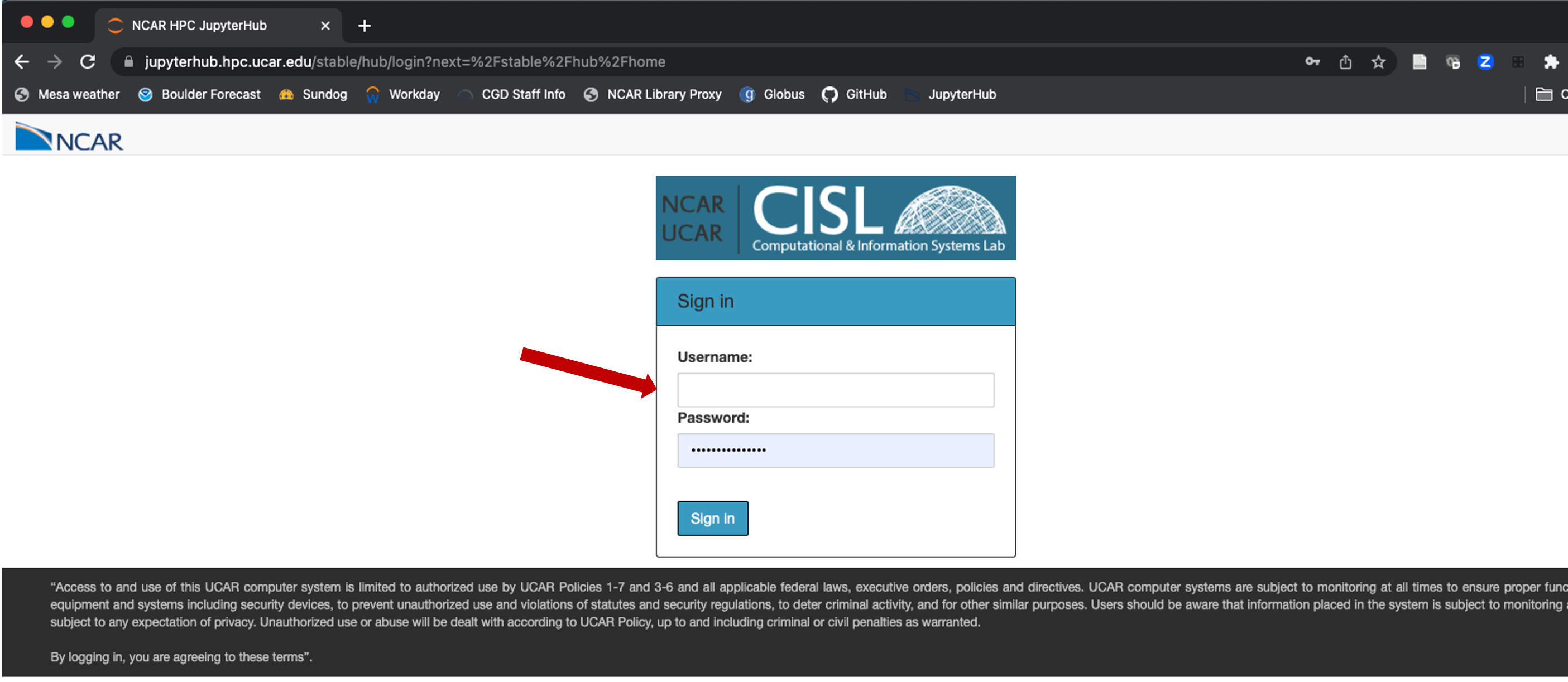
Go to the JupyterHub website (https://jupyterhub.hpc.ucar.edu/) and click on the “Production” button.

This will take you to a page where you enter your username and password, exactly as you do to login to Cheyenne or Casper. After you do this and click “Sign In” you will get a Duo verification request as well.

Start your server on JupyterHub.

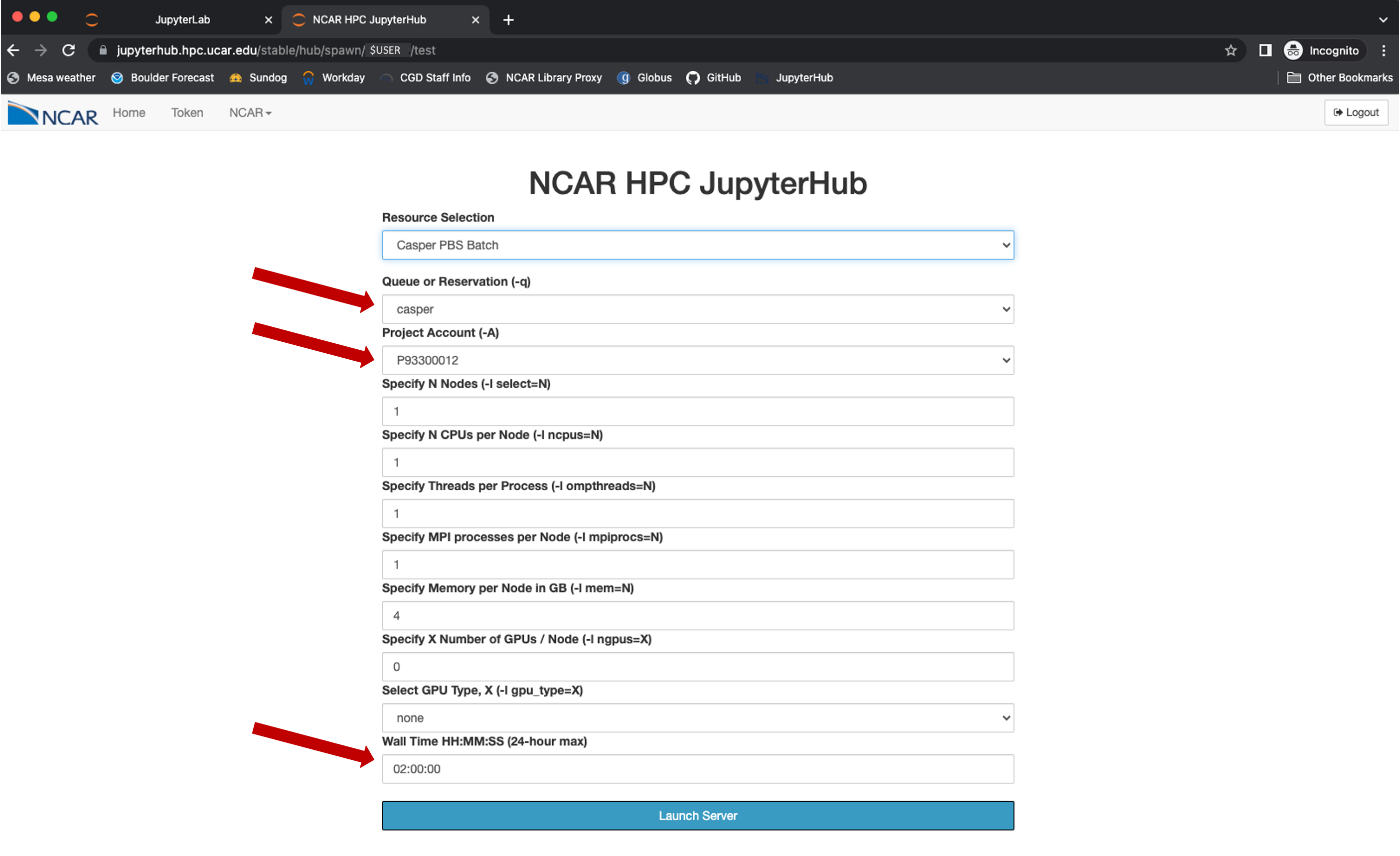
Select the “Casper PBS Batch” option in the drop down menu.

After selecting “Casper PBS Batch” you need to make other choices to select the right resources. You should use the queue and project account keys specified below. You may also want to request 03:00:00 for your Wall Time so that your server is active for the entire hands-on activity session. Do not change any other selection for this tutorial. If you are doing further analysis of model experiments you may need to change these settings and can find more information at the CISL Documentation about JupyterHub.

You may have to wait a moment or two for your server to start up.

Your JupyterHub session is now active and ready to run.
Step 3. Open a Diagnostics Notebook#
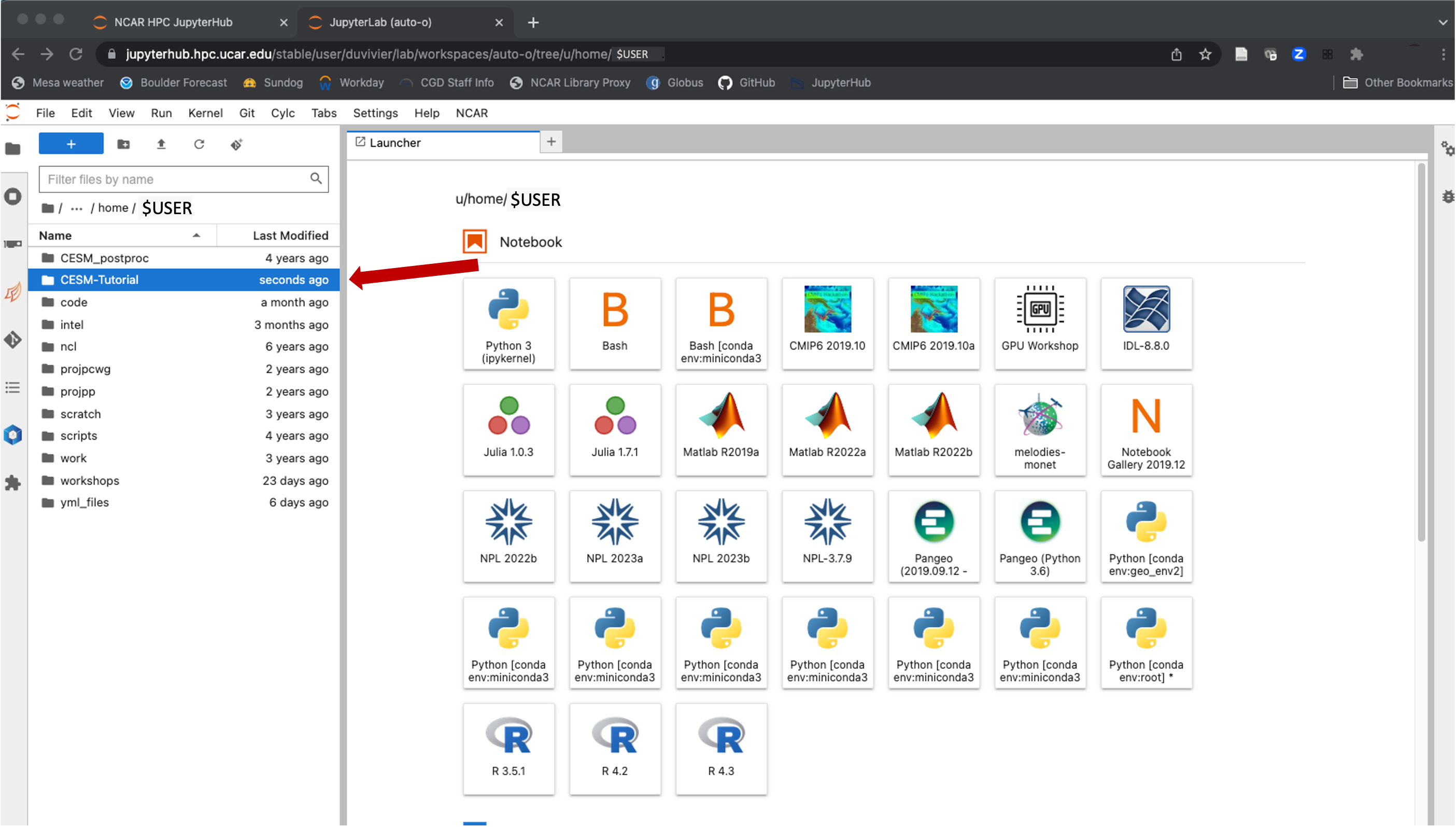
When your JupyterHub session opens you should be in your home directory on the NCAR HPC. In Step 1 you cloned the “CESM-Tutorial” repository, which has the notebooks you will run in this activity.

To get to the Diagnostics notebooks, double click the following sequence of folders:
CESM-Tutorial
notebooks
diagnostics
Click on the folder for the model component that you are interested in running (e.g. cam)
Click on the
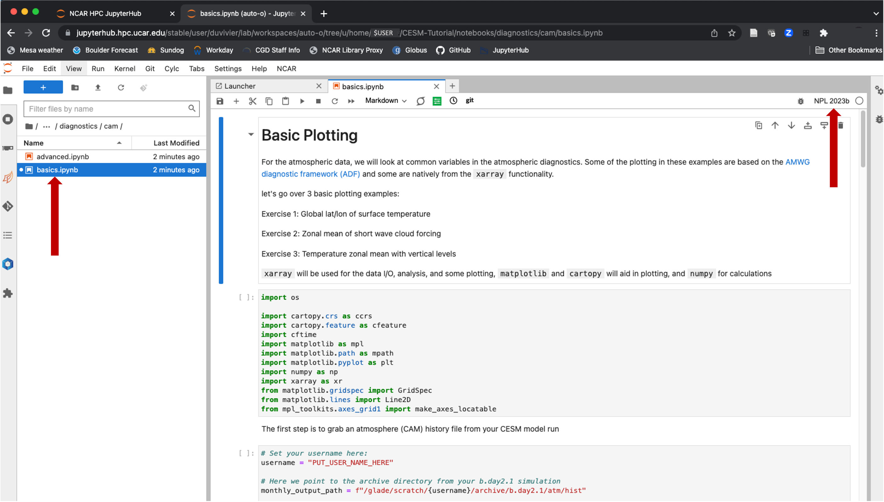
basics.ipynbnotebook (see arrow on left, below)
The final path in your browser url line for the following example should be:
$USER/CESM-Tutorial/notebooks/diagnostics/cam/basics.ipynb

Step 4. Check Your Notebook Kernel#
Check your kernel (see arrow in upper right corner, above). It should be either NPL 2023a or NPL 2023b. You should use the specified kernel for any diagnostics you do during the tutorial as it is a default environment available on NCAR HPC and the notebooks here have been tested so that they work with that particular kernel for the analysis environment. We have set the default kernels and specifiy what they should be in each component notebook. However, if you need to change it click on the kernel button and select the correct kernel.
Step 5. Run Jupyter Notebook Cells#
To run a Jupyter cell
Type your command into the cell
To execute the command:
Press shift+return
OR- Select the cell then click the 'play' button at the top of the window (see red arrow, above)All figures will be rendered in the Jupyter Notebook, so there is no need to open any other window for this portion of the lab activities.
