Regridding High Resolution Observations to a High Resolution Model Grid#
In this example, we will cover how to leverage a useful package from the Pangeo Ecosystem, xESMF. One important note when using this package, is make sure you are using the most up-to-date documentation/version, a few years ago, development moved to the pangeo-data branch of the package, installable using the following:
conda install -c conda-forge xESMF
Imports#
import ast

import cf_xarray
import cftime
import geocat.comp
import holoviews as hv
import hvplot
import hvplot.xarray
import intake
import numpy as np
import pop_tools
import xarray as xr
import xesmf as xe
from distributed import Client
from ncar_jobqueue import NCARCluster
from pop_tools.grid import _compute_corners

hv.extension('bokeh')


cluster = NCARCluster(memory='20 GB')
cluster.scale(20)
client = Client(cluster)
client
Client
Client-43aadd5b-1240-11ec-9327-3cecef1b11de
| Connection method: Cluster object | Cluster type: dask_jobqueue.PBSCluster |
| Dashboard: https://jupyterhub.hpc.ucar.edu/stable/user/mgrover/proxy/8787/status |
Cluster Info
PBSCluster
a49fcaa9
| Dashboard: https://jupyterhub.hpc.ucar.edu/stable/user/mgrover/proxy/8787/status | Workers: 0 |
| Total threads: 0 | Total memory: 0 B |
Scheduler Info
Scheduler
Scheduler-d92edee1-f368-4baf-9801-ff91a4a71464
| Comm: tcp://10.12.206.51:34462 | Workers: 0 |
| Dashboard: https://jupyterhub.hpc.ucar.edu/stable/user/mgrover/proxy/8787/status | Total threads: 0 |
| Started: Just now | Total memory: 0 B |
Workers
Read in Observational Data from the World Ocean Atlas#
For this example, we will download a file from the World Ocean Atlas, which includes a variety of ocean observations assembled from the World Ocean Database.
These observations have been gridded to a global grid at a variety of resolutions, including:
5 degree
1 degree
0.25 degree
Only a few variables are available at 0.25 degree resolution, so in this example, we will look at Temperature since that is a field that is in our output and we are using high resolution (0.1 degree) output.
!wget https://www.ncei.noaa.gov/data/oceans/woa/WOA18/DATA/temperature/netcdf/decav/0.25/woa18_decav_t01_04.nc
--2021-09-10 08:06:50--  https://www.ncei.noaa.gov/data/oceans/woa/WOA18/DATA/temperature/netcdf/decav/0.25/woa18_decav_t01_04.nc
Resolving www.ncei.noaa.gov... 205.167.25.172, 205.167.25.171, 205.167.25.167, ...
Connecting to www.ncei.noaa.gov|205.167.25.172|:443... connected.
HTTP request sent, awaiting response... 200 OK
Length: 427712938 (408M) [application/x-netcdf]
Saving to: ‘woa18_decav_t01_04.nc.1’

woa18_decav_t01_04. 100%[===================>] 407.90M  52.9MB/s    in 8.0s

2021-09-10 08:06:58 (50.9 MB/s) - ‘woa18_decav_t01_04.nc.1’ saved [427712938/427712938]
The Pangeo-Forge Method#
One could also use an example from the Pangeo-Forge documentation to accomplish this data-access task, since there is a “recipe” for using data from the World Ocean Atlas.
I suggest following that documentation, and in the “Define the File Pattern” section, replace the format_function with the following:
def format_function(variable, time):
    return ("https://www.ncei.noaa.gov/thredds-ocean/fileServer/ncei/woa/"
            f"{variable}/decav/0.25/woa18_decav_{variable[0]}{time:02d}_04.nc")
In the original example, they were looking at the 5 degree output; whereas in this example, we are interested in the 0.25 degree data - fortunately, it is an easy fix!
Read in the Data using Xarray#
We need to specify decode_times = False here since the times can be a bit difficult to work with. The calendar units have units months since 1955-01-01 00:00:00, but effectively, this dataset is a set of decadal averages (decav), for the month of January (01)
obs_ds = xr.open_dataset('woa18_decav_t01_04.nc', decode_times=False)
obs_ds
<xarray.Dataset>
Dimensions:             (lat: 720, nbounds: 2, lon: 1440, depth: 57, time: 1)
Coordinates:
  * lat                 (lat) float32 -89.88 -89.62 -89.38 ... 89.38 89.62 89.88
  * lon                 (lon) float32 -179.9 -179.6 -179.4 ... 179.4 179.6 179.9
  * depth               (depth) float32 0.0 5.0 10.0 ... 1.45e+03 1.5e+03
  * time                (time) float32 372.5
Dimensions without coordinates: nbounds
Data variables: (12/13)
    crs                 int32 -2147483647
    lat_bnds            (lat, nbounds) float32 -90.0 -89.75 ... 89.75 90.0
    lon_bnds            (lon, nbounds) float32 -180.0 -179.8 ... 179.8 180.0
    depth_bnds          (depth, nbounds) float32 0.0 2.5 ... 1.475e+03 1.5e+03
    climatology_bounds  (time, nbounds) float32 0.0 404.0
    t_an                (time, depth, lat, lon) float32 ...
    ...                  ...
    t_dd                (time, depth, lat, lon) float64 ...
    t_sd                (time, depth, lat, lon) float32 ...
    t_se                (time, depth, lat, lon) float32 ...
    t_oa                (time, depth, lat, lon) float32 ...
    t_ma                (time, depth, lat, lon) float32 ...
    t_gp                (time, depth, lat, lon) float64 ...
Attributes: (12/49)
    Conventions:                     CF-1.6, ACDD-1.3
    title:                           World Ocean Atlas 2018 : sea_water_tempe...
    summary:                         Climatological mean temperature for the ...
    references:                      Locarnini, R. A., A. V. Mishonov, O. K. ...
    institution:                     National Centers for Environmental Infor...
    comment:                         global climatology as part of the World ...
    ...                              ...
    publisher_email:                 NCEI.info@noaa.gov
    nodc_template_version:           NODC_NetCDF_Grid_Template_v2.0
    license:                         These data are openly available to the p...
    metadata_link:                   https://www.nodc.noaa.gov/OC5/woa18/
    date_created:                    2019-07-29
date_modified: 2019-07-29 - lat: 720
- nbounds: 2
- lon: 1440
- depth: 57
- time: 1
- lat(lat)float32-89.88 -89.62 ... 89.62 89.88
- standard_name :
- latitude
- long_name :
- latitude
- units :
- degrees_north
- axis :
- Y
- bounds :
- lat_bnds
array([-89.875, -89.625, -89.375, ..., 89.375, 89.625, 89.875], dtype=float32) - lon(lon)float32-179.9 -179.6 ... 179.6 179.9
- standard_name :
- longitude
- long_name :
- longitude
- units :
- degrees_east
- axis :
- X
- bounds :
- lon_bnds
array([-179.875, -179.625, -179.375, ..., 179.375, 179.625, 179.875], dtype=float32) - depth(depth)float320.0 5.0 10.0 ... 1.45e+03 1.5e+03
- standard_name :
- depth
- bounds :
- depth_bnds
- positive :
- down
- units :
- meters
- axis :
- Z
array([ 0., 5., 10., 15., 20., 25., 30., 35., 40., 45., 50., 55., 60., 65., 70., 75., 80., 85., 90., 95., 100., 125., 150., 175., 200., 225., 250., 275., 300., 325., 350., 375., 400., 425., 450., 475., 500., 550., 600., 650., 700., 750., 800., 850., 900., 950., 1000., 1050., 1100., 1150., 1200., 1250., 1300., 1350., 1400., 1450., 1500.], dtype=float32) - time(time)float32372.5
- standard_name :
- time
- long_name :
- time
- units :
- months since 1955-01-01 00:00:00
- axis :
- T
- climatology :
- climatology_bounds
array([372.5], dtype=float32)
- crs()int32...
- grid_mapping_name :
- latitude_longitude
- epsg_code :
- EPSG:4326
- longitude_of_prime_meridian :
- 0.0
- semi_major_axis :
- 6378137.0
- inverse_flattening :
- 298.25723
array(-2147483647, dtype=int32)
- lat_bnds(lat, nbounds)float32...
- comment :
- latitude bounds
array([[-90. , -89.75], [-89.75, -89.5 ], [-89.5 , -89.25], ..., [ 89.25, 89.5 ], [ 89.5 , 89.75], [ 89.75, 90. ]], dtype=float32) - lon_bnds(lon, nbounds)float32...
- comment :
- longitude bounds
array([[-180. , -179.75], [-179.75, -179.5 ], [-179.5 , -179.25], ..., [ 179.25, 179.5 ], [ 179.5 , 179.75], [ 179.75, 180. ]], dtype=float32) - depth_bnds(depth, nbounds)float32...
- comment :
- depth bounds
array([[ 0. , 2.5], [ 2.5, 7.5], [ 7.5, 12.5], [ 12.5, 17.5], [ 17.5, 22.5], [ 22.5, 27.5], [ 27.5, 32.5], [ 32.5, 37.5], [ 37.5, 42.5], [ 42.5, 47.5], [ 47.5, 52.5], [ 52.5, 57.5], [ 57.5, 62.5], [ 62.5, 67.5], [ 67.5, 72.5], [ 72.5, 77.5], [ 77.5, 82.5], [ 82.5, 87.5], [ 87.5, 92.5], [ 92.5, 97.5], [ 97.5, 112.5], [ 112.5, 137.5], [ 137.5, 162.5], [ 162.5, 187.5], [ 187.5, 212.5], [ 212.5, 237.5], [ 237.5, 262.5], [ 262.5, 287.5], [ 287.5, 312.5], [ 312.5, 337.5], [ 337.5, 362.5], [ 362.5, 387.5], [ 387.5, 412.5], [ 412.5, 437.5], [ 437.5, 462.5], [ 462.5, 487.5], [ 487.5, 525. ], [ 525. , 575. ], [ 575. , 625. ], [ 625. , 675. ], [ 675. , 725. ], [ 725. , 775. ], [ 775. , 825. ], [ 825. , 875. ], [ 875. , 925. ], [ 925. , 975. ], [ 975. , 1025. ], [1025. , 1075. ], [1075. , 1125. ], [1125. , 1175. ], [1175. , 1225. ], [1225. , 1275. ], [1275. , 1325. ], [1325. , 1375. ], [1375. , 1425. ], [1425. , 1475. ], [1475. , 1500. ]], dtype=float32) - climatology_bounds(time, nbounds)float32...
- comment :
- This variable defines the bounds of the climatological time period for each time
array([[ 0., 404.]], dtype=float32)
- t_an(time, depth, lat, lon)float32...
- standard_name :
- sea_water_temperature
- long_name :
- Objectively analyzed mean fields for sea_water_temperature at standard depth levels.
- cell_methods :
- area: mean depth: mean time: mean within years time: mean over years
- grid_mapping :
- crs
- units :
- degrees_celsius
[59097600 values with dtype=float32]
- t_mn(time, depth, lat, lon)float32...
- standard_name :
- sea_water_temperature
- long_name :
- Average of all unflagged interpolated values at each standard depth level for sea_water_temperature in each grid-square which contain at least one measurement.
- cell_methods :
- area: mean depth: mean time: mean within years time: mean over years
- grid_mapping :
- crs
- units :
- degrees_celsius
[59097600 values with dtype=float32]
- t_dd(time, depth, lat, lon)float64...
- standard_name :
- sea_water_temperature number_of_observations
- long_name :
- The number of observations of sea_water_temperature in each grid-square at each standard depth level.
- cell_methods :
- area: sum depth: point time: sum
- grid_mapping :
- crs
- units :
- 1
[59097600 values with dtype=float64]
- t_sd(time, depth, lat, lon)float32...
- long_name :
- The standard deviation about the statistical mean of sea_water_temperature in each grid-square at each standard depth level.
- cell_methods :
- area: mean depth: mean time: standard_deviation
- grid_mapping :
- crs
- units :
- degrees_celsius
[59097600 values with dtype=float32]
- t_se(time, depth, lat, lon)float32...
- standard_name :
- sea_water_temperature standard_error
- long_name :
- The standard error about the statistical mean of sea_water_temperature in each grid-square at each standard depth level.
- cell_methods :
- area: mean depth: mean time: mean
- grid_mapping :
- crs
- units :
- degrees_celsius
[59097600 values with dtype=float32]
- t_oa(time, depth, lat, lon)float32...
- standard_name :
- sea_water_temperature
- long_name :
- statistical mean value minus the objectively analyzed mean value for sea_water_temperature.
- cell_methods :
- area: mean depth: mean time: mean with years time: mean over years
- grid_mapping :
- crs
- units :
- degrees_celsius
[59097600 values with dtype=float32]
- t_ma(time, depth, lat, lon)float32...
- standard_name :
- sea_water_temperature
- long_name :
- The objectively analyzed value for the given time period minus the objectively analyzed annual mean value for sea_water_temperature.
- cell_methods :
- area: mean depth: mean time: mean within years time: mean over years
- grid_mapping :
- crs
- units :
- degrees_celsius
[59097600 values with dtype=float32]
- t_gp(time, depth, lat, lon)float64...
- long_name :
- The number of grid-squares within the smallest radius of influence around each grid-square which contain a statistical mean for sea_water_temperature.
- cell_methods :
- area: mean depth: mean time: mean within years time: mean over years
- grid_mapping :
- crs
- units :
- 1
[59097600 values with dtype=float64]
- Conventions :
- CF-1.6, ACDD-1.3
- title :
- World Ocean Atlas 2018 : sea_water_temperature January 1955-2017 0.25 degree
- summary :
- Climatological mean temperature for the global ocean from in situ profile data
- references :
- Locarnini, R. A., A. V. Mishonov, O. K. Baranova, T. P. Boyer, M. M. Zweng, H. E. Garcia, J. R. Reagan, D. Seidov, K. W. Weathers, C. R. Paver, I. V. Smolyar, 2019: World Ocean Atlas 2018, Volume 1: Temperature. A. V. Mishonov, Technical Ed., NOAA Atlas NESDIS 81
- institution :
- National Centers for Environmental Information (NCEI)
- comment :
- global climatology as part of the World Ocean Atlas project
- id :
- woa18_decav_t01_04.nc
- naming_authority :
- gov.noaa.ncei
- sea_name :
- World-Wide Distribution
- time_coverage_start :
- 1955-01-01
- time_coverage_end :
- 2017-01-31
- time_coverage_duration :
- P63Y
- time_coverage_resolution :
- P01M
- geospatial_lat_min :
- -90.0
- geospatial_lat_max :
- 90.0
- geospatial_lon_min :
- -180.0
- geospatial_lon_max :
- 180.0
- geospatial_vertical_min :
- 0.0
- geospatial_vertical_max :
- 1500.0
- geospatial_lat_units :
- degrees_north
- geospatial_lat_resolution :
- 0.25 degrees
- geospatial_lon_units :
- degrees_east
- geospatial_lon_resolution :
- 0.25 degrees
- geospatial_vertical_units :
- m
- geospatial_vertical_resolution :
- SPECIAL
- geospatial_vertical_positive :
- down
- creator_name :
- Ocean Climate Laboratory
- creator_email :
- NCEI.info@noaa.gov
- creator_url :
- http://www.ncei.noaa.gov
- creator_type :
- group
- creator_institution :
- National Centers for Environmental Information
- project :
- World Ocean Atlas Project
- processing_level :
- processed
- keywords :
- Oceans< Ocean Temperature > Water Temperature
- keywords_vocabulary :
- ISO 19115
- standard_name_vocabulary :
- CF Standard Name Table v49
- contributor_name :
- Ocean Climate Laboratory
- contributor_role :
- Calculation of climatologies
- cdm_data_type :
- Grid
- publisher_name :
- National Centers for Environmental Information (NCEI)
- publisher_institution :
- National Centers for Environmental Information
- publisher_type :
- institution
- publisher_url :
- http://www.ncei.noaa.gov/
- publisher_email :
- NCEI.info@noaa.gov
- nodc_template_version :
- NODC_NetCDF_Grid_Template_v2.0
- license :
- These data are openly available to the public. Please acknowledge the use of these data with the text given in the acknowledgment attribute.
- metadata_link :
- https://www.nodc.noaa.gov/OC5/woa18/
- date_created :
- 2019-07-29
- date_modified :
- 2019-07-29
You’ll notice several temperature variables, with the variables using the notation t_{}, for example, t_an is the average temperature over that period. This is the variable we are most interested, and we can change the name of that variable to reflect the naming convention in the POP ocean model - TEMP
obs_ds.t_an
<xarray.DataArray 't_an' (time: 1, depth: 57, lat: 720, lon: 1440)>
[59097600 values with dtype=float32]
Coordinates:
  * lat      (lat) float32 -89.88 -89.62 -89.38 -89.12 ... 89.38 89.62 89.88
  * lon      (lon) float32 -179.9 -179.6 -179.4 -179.1 ... 179.4 179.6 179.9
  * depth    (depth) float32 0.0 5.0 10.0 15.0 ... 1.4e+03 1.45e+03 1.5e+03
  * time     (time) float32 372.5
Attributes:
    standard_name:  sea_water_temperature
    long_name:      Objectively analyzed mean fields for sea_water_temperatur...
    cell_methods:   area: mean depth: mean time: mean within years time: mean...
    grid_mapping:   crs
units: degrees_celsius- time: 1
- depth: 57
- lat: 720
- lon: 1440
- ...
[59097600 values with dtype=float32]
- lat(lat)float32-89.88 -89.62 ... 89.62 89.88
- standard_name :
- latitude
- long_name :
- latitude
- units :
- degrees_north
- axis :
- Y
- bounds :
- lat_bnds
array([-89.875, -89.625, -89.375, ..., 89.375, 89.625, 89.875], dtype=float32) - lon(lon)float32-179.9 -179.6 ... 179.6 179.9
- standard_name :
- longitude
- long_name :
- longitude
- units :
- degrees_east
- axis :
- X
- bounds :
- lon_bnds
array([-179.875, -179.625, -179.375, ..., 179.375, 179.625, 179.875], dtype=float32) - depth(depth)float320.0 5.0 10.0 ... 1.45e+03 1.5e+03
- standard_name :
- depth
- bounds :
- depth_bnds
- positive :
- down
- units :
- meters
- axis :
- Z
array([ 0., 5., 10., 15., 20., 25., 30., 35., 40., 45., 50., 55., 60., 65., 70., 75., 80., 85., 90., 95., 100., 125., 150., 175., 200., 225., 250., 275., 300., 325., 350., 375., 400., 425., 450., 475., 500., 550., 600., 650., 700., 750., 800., 850., 900., 950., 1000., 1050., 1100., 1150., 1200., 1250., 1300., 1350., 1400., 1450., 1500.], dtype=float32) - time(time)float32372.5
- standard_name :
- time
- long_name :
- time
- units :
- months since 1955-01-01 00:00:00
- axis :
- T
- climatology :
- climatology_bounds
array([372.5], dtype=float32)
- standard_name :
- sea_water_temperature
- long_name :
- Objectively analyzed mean fields for sea_water_temperature at standard depth levels.
- cell_methods :
- area: mean depth: mean time: mean within years time: mean over years
- grid_mapping :
- crs
- units :
- degrees_celsius
We can also subset for just TEMP here, in addition to the bounds information, which can be utilized by xESMF during regridding.
obs_ds = obs_ds.rename({'t_an': 'TEMP'})[['TEMP', 'lat_bnds', 'lon_bnds']]
obs_ds
<xarray.Dataset>
Dimensions:   (time: 1, depth: 57, lat: 720, lon: 1440, nbounds: 2)
Coordinates:
  * lat       (lat) float32 -89.88 -89.62 -89.38 -89.12 ... 89.38 89.62 89.88
  * lon       (lon) float32 -179.9 -179.6 -179.4 -179.1 ... 179.4 179.6 179.9
  * depth     (depth) float32 0.0 5.0 10.0 15.0 ... 1.4e+03 1.45e+03 1.5e+03
  * time      (time) float32 372.5
Dimensions without coordinates: nbounds
Data variables:
    TEMP      (time, depth, lat, lon) float32 ...
    lat_bnds  (lat, nbounds) float32 -90.0 -89.75 -89.75 ... 89.75 89.75 90.0
    lon_bnds  (lon, nbounds) float32 -180.0 -179.8 -179.8 ... 179.8 179.8 180.0
Attributes: (12/49)
    Conventions:                     CF-1.6, ACDD-1.3
    title:                           World Ocean Atlas 2018 : sea_water_tempe...
    summary:                         Climatological mean temperature for the ...
    references:                      Locarnini, R. A., A. V. Mishonov, O. K. ...
    institution:                     National Centers for Environmental Infor...
    comment:                         global climatology as part of the World ...
    ...                              ...
    publisher_email:                 NCEI.info@noaa.gov
    nodc_template_version:           NODC_NetCDF_Grid_Template_v2.0
    license:                         These data are openly available to the p...
    metadata_link:                   https://www.nodc.noaa.gov/OC5/woa18/
    date_created:                    2019-07-29
date_modified: 2019-07-29 - time: 1
- depth: 57
- lat: 720
- lon: 1440
- nbounds: 2
- lat(lat)float32-89.88 -89.62 ... 89.62 89.88
- standard_name :
- latitude
- long_name :
- latitude
- units :
- degrees_north
- axis :
- Y
- bounds :
- lat_bnds
array([-89.875, -89.625, -89.375, ..., 89.375, 89.625, 89.875], dtype=float32) - lon(lon)float32-179.9 -179.6 ... 179.6 179.9
- standard_name :
- longitude
- long_name :
- longitude
- units :
- degrees_east
- axis :
- X
- bounds :
- lon_bnds
array([-179.875, -179.625, -179.375, ..., 179.375, 179.625, 179.875], dtype=float32) - depth(depth)float320.0 5.0 10.0 ... 1.45e+03 1.5e+03
- standard_name :
- depth
- bounds :
- depth_bnds
- positive :
- down
- units :
- meters
- axis :
- Z
array([ 0., 5., 10., 15., 20., 25., 30., 35., 40., 45., 50., 55., 60., 65., 70., 75., 80., 85., 90., 95., 100., 125., 150., 175., 200., 225., 250., 275., 300., 325., 350., 375., 400., 425., 450., 475., 500., 550., 600., 650., 700., 750., 800., 850., 900., 950., 1000., 1050., 1100., 1150., 1200., 1250., 1300., 1350., 1400., 1450., 1500.], dtype=float32) - time(time)float32372.5
- standard_name :
- time
- long_name :
- time
- units :
- months since 1955-01-01 00:00:00
- axis :
- T
- climatology :
- climatology_bounds
array([372.5], dtype=float32)
- TEMP(time, depth, lat, lon)float32...
- standard_name :
- sea_water_temperature
- long_name :
- Objectively analyzed mean fields for sea_water_temperature at standard depth levels.
- cell_methods :
- area: mean depth: mean time: mean within years time: mean over years
- grid_mapping :
- crs
- units :
- degrees_celsius
[59097600 values with dtype=float32]
- lat_bnds(lat, nbounds)float32-90.0 -89.75 -89.75 ... 89.75 90.0
- comment :
- latitude bounds
array([[-90. , -89.75], [-89.75, -89.5 ], [-89.5 , -89.25], ..., [ 89.25, 89.5 ], [ 89.5 , 89.75], [ 89.75, 90. ]], dtype=float32) - lon_bnds(lon, nbounds)float32-180.0 -179.8 ... 179.8 180.0
- comment :
- longitude bounds
array([[-180.  , -179.75],
       [-179.75, -179.5 ],
       [-179.5 , -179.25],
       ...,
       [ 179.25,  179.5 ],
       [ 179.5 ,  179.75],
       [ 179.75,  180.  ]], dtype=float32)
- Conventions :
- CF-1.6, ACDD-1.3
- title :
- World Ocean Atlas 2018 : sea_water_temperature January 1955-2017 0.25 degree
- summary :
- Climatological mean temperature for the global ocean from in situ profile data
- references :
- Locarnini, R. A., A. V. Mishonov, O. K. Baranova, T. P. Boyer, M. M. Zweng, H. E. Garcia, J. R. Reagan, D. Seidov, K. W. Weathers, C. R. Paver, I. V. Smolyar, 2019: World Ocean Atlas 2018, Volume 1: Temperature. A. V. Mishonov, Technical Ed., NOAA Atlas NESDIS 81
- institution :
- National Centers for Environmental Information (NCEI)
- comment :
- global climatology as part of the World Ocean Atlas project
- id :
- woa18_decav_t01_04.nc
- naming_authority :
- gov.noaa.ncei
- sea_name :
- World-Wide Distribution
- time_coverage_start :
- 1955-01-01
- time_coverage_end :
- 2017-01-31
- time_coverage_duration :
- P63Y
- time_coverage_resolution :
- P01M
- geospatial_lat_min :
- -90.0
- geospatial_lat_max :
- 90.0
- geospatial_lon_min :
- -180.0
- geospatial_lon_max :
- 180.0
- geospatial_vertical_min :
- 0.0
- geospatial_vertical_max :
- 1500.0
- geospatial_lat_units :
- degrees_north
- geospatial_lat_resolution :
- 0.25 degrees
- geospatial_lon_units :
- degrees_east
- geospatial_lon_resolution :
- 0.25 degrees
- geospatial_vertical_units :
- m
- geospatial_vertical_resolution :
- SPECIAL
- geospatial_vertical_positive :
- down
- creator_name :
- Ocean Climate Laboratory
- creator_email :
- NCEI.info@noaa.gov
- creator_url :
- http://www.ncei.noaa.gov
- creator_type :
- group
- creator_institution :
- National Centers for Environmental Information
- project :
- World Ocean Atlas Project
- processing_level :
- processed
- keywords :
- Oceans< Ocean Temperature > Water Temperature
- keywords_vocabulary :
- ISO 19115
- standard_name_vocabulary :
- CF Standard Name Table v49
- contributor_name :
- Ocean Climate Laboratory
- contributor_role :
- Calculation of climatologies
- cdm_data_type :
- Grid
- publisher_name :
- National Centers for Environmental Information (NCEI)
- publisher_institution :
- National Centers for Environmental Information
- publisher_type :
- institution
- publisher_url :
- http://www.ncei.noaa.gov/
- publisher_email :
- NCEI.info@noaa.gov
- nodc_template_version :
- NODC_NetCDF_Grid_Template_v2.0
- license :
- These data are openly available to the public. Please acknowledge the use of these data with the text given in the acknowledgment attribute.
- metadata_link :
- https://www.nodc.noaa.gov/OC5/woa18/
- date_created :
- 2019-07-29
- date_modified :
- 2019-07-29
Read in Model Data#
In this example, we are using high resolution ocean model output from CESM. This data is stored on the GLADE filesystem on NCAR HPC resources. Here is a repository describing how we generated a catalog similar to this, with some examples of plotting the data
data_catalog = intake.open_esm_datastore(
    "/glade/work/mgrover/hires-fulljra-catalog.json",
    csv_kwargs={"converters": {"variables": ast.literal_eval}},
    sep="/",
)
data_catalog
None catalog with 4 dataset(s) from 2765 asset(s):
| unique | |
|---|---|
| component | 1 |
| stream | 2 |
| date | 2694 |
| case | 2 |
| member_id | 2 |
| frequency | 3 |
| variables | 97 |
| path | 2765 |
Let’s subset for temperature (TEMP) here
data_catalog_subset = data_catalog.search(variables='TEMP')
When reading in the data, we are chunking by horizontal, and vertical dimensions, since we will be taking a temporal average in future steps. Chunking by dimensions not being averaged over helps reduced the amount of data on disk that is moved around during computation.
dsets = data_catalog_subset.to_dataset_dict(
    cdf_kwargs={'chunks': {'nlat': 800, 'nlon': 900, 'z_t': 4}}
)
--> The keys in the returned dictionary of datasets are constructed as follows:
	'component/stream/case'
dsets.keys()
dict_keys(['ocn/pop.h/g.e20.G.TL319_t13.control.001', 'ocn/pop.h/g.e20.G.TL319_t13.control.001_hfreq'])
Subset for time - here, we are interested in year 24 through 53#
The model begins at 1958, so this roughly corresponds to 1981-2010, which is when the climatology from WOA was calculated
We choose February from year 24 through January of year 53 since the time represents the end of the time bounds
start_time = cftime.datetime(24, 2, 1, 0, 0, 0, 0, calendar='noleap', has_year_zero=True)
end_time = cftime.datetime(53, 1, 1, 0, 0, 0, 0, calendar='noleap', has_year_zero=True)
dset_list = []

for key in dsets.keys():
    dset_list.append(dsets[key].sel(time=slice(start_time, end_time)))
model_ds = xr.concat(
    dset_list, dim='time', data_vars="minimal", coords="minimal", compat="override"
)
It looks like the model does not include the entire time range (up to ~2005), but it is pretty close!
model_ds
<xarray.Dataset>
Dimensions:  (time: 1764, z_t: 62, nlat: 2400, nlon: 3600)
Coordinates:
  * time     (time) object 0024-02-01 00:00:00 ... 0049-11-02 00:00:00
  * z_t      (z_t) float32 500.0 1.5e+03 2.5e+03 ... 5.625e+05 5.875e+05
    ULONG    (nlat, nlon) float64 dask.array<chunksize=(800, 900), meta=np.ndarray>
    ULAT     (nlat, nlon) float64 dask.array<chunksize=(800, 900), meta=np.ndarray>
    TLONG    (nlat, nlon) float64 dask.array<chunksize=(800, 900), meta=np.ndarray>
    TLAT     (nlat, nlon) float64 dask.array<chunksize=(800, 900), meta=np.ndarray>
Dimensions without coordinates: nlat, nlon
Data variables:
    TEMP     (time, z_t, nlat, nlon) float32 dask.array<chunksize=(1, 4, 800, 900), meta=np.ndarray>
Attributes:
    cell_methods:            cell_methods = time: mean ==> the variable value...
    time_period_freq:        month_1
    contents:                Diagnostic and Prognostic Variables
    calendar:                All years have exactly  365 days.
    source:                  CCSM POP2, the CCSM Ocean Component
    history:                 none
    model_doi_url:           https://doi.org/10.5065/D67H1H0V
    Conventions:             CF-1.0; http://www.cgd.ucar.edu/cms/eaton/netcdf...
    intake_esm_varname:      ['TEMP']
    revision:                $Id: tavg.F90 89091 2018-04-30 15:58:32Z altunta...
    title:                   g.e20.G.TL319_t13.control.001
intake_esm_dataset_key: ocn/pop.h/g.e20.G.TL319_t13.control.001- time: 1764
- z_t: 62
- nlat: 2400
- nlon: 3600
- time(time)object0024-02-01 00:00:00 ... 0049-11-...
- long_name :
- time
- bounds :
- time_bound
array([cftime.datetime(24, 2, 1, 0, 0, 0, 0, calendar='noleap', has_year_zero=True), cftime.datetime(24, 3, 1, 0, 0, 0, 0, calendar='noleap', has_year_zero=True), cftime.datetime(24, 4, 1, 0, 0, 0, 0, calendar='noleap', has_year_zero=True), ..., cftime.datetime(49, 10, 23, 0, 0, 0, 0, calendar='noleap', has_year_zero=True), cftime.datetime(49, 10, 28, 0, 0, 0, 0, calendar='noleap', has_year_zero=True), cftime.datetime(49, 11, 2, 0, 0, 0, 0, calendar='noleap', has_year_zero=True)], dtype=object) - z_t(z_t)float32500.0 1.5e+03 ... 5.875e+05
- long_name :
- depth from surface to midpoint of layer
- units :
- centimeters
- positive :
- down
- valid_min :
- 500.0
- valid_max :
- 587499.06
array([5.000000e+02, 1.500000e+03, 2.500000e+03, 3.500000e+03, 4.500000e+03, 5.500000e+03, 6.500000e+03, 7.500000e+03, 8.500000e+03, 9.500000e+03, 1.050000e+04, 1.150000e+04, 1.250000e+04, 1.350000e+04, 1.450000e+04, 1.550000e+04, 1.650984e+04, 1.754790e+04, 1.862913e+04, 1.976603e+04, 2.097114e+04, 2.225783e+04, 2.364088e+04, 2.513702e+04, 2.676542e+04, 2.854837e+04, 3.051192e+04, 3.268680e+04, 3.510935e+04, 3.782276e+04, 4.087846e+04, 4.433777e+04, 4.827367e+04, 5.277280e+04, 5.793729e+04, 6.388626e+04, 7.075633e+04, 7.870025e+04, 8.788252e+04, 9.847059e+04, 1.106204e+05, 1.244567e+05, 1.400497e+05, 1.573946e+05, 1.764003e+05, 1.968944e+05, 2.186457e+05, 2.413972e+05, 2.649001e+05, 2.889385e+05, 3.133405e+05, 3.379793e+05, 3.627670e+05, 3.876452e+05, 4.125768e+05, 4.375392e+05, 4.625190e+05, 4.875083e+05, 5.125028e+05, 5.375000e+05, 5.624991e+05, 5.874991e+05], dtype=float32) - ULONG(nlat, nlon)float64dask.array<chunksize=(800, 900), meta=np.ndarray>
- long_name :
- array of u-grid longitudes
- units :
- degrees_east
Array Chunk Bytes 65.92 MiB 5.49 MiB Shape (2400, 3600) (800, 900) Count 13 Tasks 12 Chunks Type float64 numpy.ndarray - ULAT(nlat, nlon)float64dask.array<chunksize=(800, 900), meta=np.ndarray>
- long_name :
- array of u-grid latitudes
- units :
- degrees_north
Array Chunk Bytes 65.92 MiB 5.49 MiB Shape (2400, 3600) (800, 900) Count 13 Tasks 12 Chunks Type float64 numpy.ndarray - TLONG(nlat, nlon)float64dask.array<chunksize=(800, 900), meta=np.ndarray>
- long_name :
- array of t-grid longitudes
- units :
- degrees_east
Array Chunk Bytes 65.92 MiB 5.49 MiB Shape (2400, 3600) (800, 900) Count 13 Tasks 12 Chunks Type float64 numpy.ndarray - TLAT(nlat, nlon)float64dask.array<chunksize=(800, 900), meta=np.ndarray>
- long_name :
- array of t-grid latitudes
- units :
- degrees_north
Array Chunk Bytes 65.92 MiB 5.49 MiB Shape (2400, 3600) (800, 900) Count 13 Tasks 12 Chunks Type float64 numpy.ndarray
- TEMP(time, z_t, nlat, nlon)float32dask.array<chunksize=(1, 4, 800, 900), meta=np.ndarray>
- long_name :
- Potential Temperature
- units :
- degC
- grid_loc :
- 3111
- cell_methods :
- time: mean
Array Chunk Bytes 3.44 TiB 10.99 MiB Shape (1764, 62, 2400, 3600) (1, 4, 800, 900) Count 1128696 Tasks 338688 Chunks Type float32 numpy.ndarray
- cell_methods :
- cell_methods = time: mean ==> the variable values are averaged over the time interval between the previous time coordinate and the current one. cell_methods absent ==> the variable values are at the time given by the current time coordinate.
- time_period_freq :
- month_1
- contents :
- Diagnostic and Prognostic Variables
- calendar :
- All years have exactly 365 days.
- source :
- CCSM POP2, the CCSM Ocean Component
- history :
- none
- model_doi_url :
- https://doi.org/10.5065/D67H1H0V
- Conventions :
- CF-1.0; http://www.cgd.ucar.edu/cms/eaton/netcdf/CF-current.htm
- intake_esm_varname :
- ['TEMP']
- revision :
- $Id: tavg.F90 89091 2018-04-30 15:58:32Z altuntas@ucar.edu $
- title :
- g.e20.G.TL319_t13.control.001
- intake_esm_dataset_key :
- ocn/pop.h/g.e20.G.TL319_t13.control.001
Compute the Monthly Mean using Geocat-Comp#
We are only interested in TEMP here, so we can subset for that when computing the climatology
model_monthly_mean = geocat.comp.climatology(model_ds[['TEMP']], 'month')
Regrid and Interpolate Vertical Levels#
As mentioned before, our observational dataset already has the bounds information, which is important for determing grid corners during the regridding process. For the POP dataset, we need to add a helper function to add this information
def gen_corner_calc(ds, cell_corner_lat='ULAT', cell_corner_lon='ULONG'):
    """
    Generates corner information and creates single dataset with output
    """

    cell_corner_lat = ds[cell_corner_lat]
    cell_corner_lon = ds[cell_corner_lon]
    # Use the function in pop-tools to get the grid corner information
    corn_lat, corn_lon = _compute_corners(cell_corner_lat, cell_corner_lon)

    # Make sure this returns four corner points
    assert corn_lon.shape[-1] == 4

    lon_shape, lat_shape = corn_lon[:, :, 0].shape
    out_shape = (lon_shape + 1, lat_shape + 1)

    # Generate numpy arrays to store destination lats/lons
    out_lons = np.zeros(out_shape)
    out_lats = np.zeros(out_shape)

    # Assign the northeast corner information
    out_lons[1:, 1:] = corn_lon[:, :, 0]
    out_lats[1:, 1:] = corn_lat[:, :, 0]

    # Assign the northwest corner information
    out_lons[1:, :-1] = corn_lon[:, :, 1]
    out_lats[1:, :-1] = corn_lat[:, :, 1]

    # Assign the southwest corner information
    out_lons[:-1, :-1] = corn_lon[:, :, 2]
    out_lats[:-1, :-1] = corn_lat[:, :, 2]

    # Assign the southeast corner information
    out_lons[:-1, 1:] = corn_lon[:, :, 3]
    out_lats[:-1, 1:] = corn_lat[:, :, 3]

    return out_lats, out_lons
lat_corners, lon_corners = gen_corner_calc(model_monthly_mean)
We can also rename our latitude and longitude names
model_monthly_mean = model_monthly_mean.rename({'TLAT': 'lat', 'TLONG': 'lon'}).drop(
    ['ULAT', 'ULONG']
)
model_monthly_mean['lon_b'] = (('nlat_b', 'nlon_b'), lon_corners)
model_monthly_mean['lat_b'] = (('nlat_b', 'nlon_b'), lat_corners)
model_monthly_mean
<xarray.Dataset>
Dimensions:  (month: 12, z_t: 62, nlat: 2400, nlon: 3600, nlat_b: 2401, nlon_b: 3601)
Coordinates:
  * month    (month) int64 1 2 3 4 5 6 7 8 9 10 11 12
  * z_t      (z_t) float64 500.0 1.5e+03 2.5e+03 ... 5.625e+05 5.875e+05
    lon      (nlat, nlon) float64 dask.array<chunksize=(800, 900), meta=np.ndarray>
    lat      (nlat, nlon) float64 dask.array<chunksize=(800, 900), meta=np.ndarray>
Dimensions without coordinates: nlat, nlon, nlat_b, nlon_b
Data variables:
    TEMP     (month, z_t, nlat, nlon) float32 dask.array<chunksize=(1, 4, 800, 900), meta=np.ndarray>
    lon_b    (nlat_b, nlon_b) float64 nan nan nan nan nan ... nan nan nan nan
    lat_b    (nlat_b, nlon_b) float64 nan nan nan nan nan ... nan nan nan nan
Attributes:
    cell_methods:            cell_methods = time: mean ==> the variable value...
    time_period_freq:        month_1
    contents:                Diagnostic and Prognostic Variables
    calendar:                All years have exactly  365 days.
    source:                  CCSM POP2, the CCSM Ocean Component
    history:                 none
    model_doi_url:           https://doi.org/10.5065/D67H1H0V
    Conventions:             CF-1.0; http://www.cgd.ucar.edu/cms/eaton/netcdf...
    intake_esm_varname:      ['TEMP']
    revision:                $Id: tavg.F90 89091 2018-04-30 15:58:32Z altunta...
    title:                   g.e20.G.TL319_t13.control.001
intake_esm_dataset_key: ocn/pop.h/g.e20.G.TL319_t13.control.001- month: 12
- z_t: 62
- nlat: 2400
- nlon: 3600
- nlat_b: 2401
- nlon_b: 3601
- month(month)int641 2 3 4 5 6 7 8 9 10 11 12
array([ 1, 2, 3, 4, 5, 6, 7, 8, 9, 10, 11, 12])
- z_t(z_t)float64500.0 1.5e+03 ... 5.875e+05
- long_name :
- depth from surface to midpoint of layer
- units :
- centimeters
- positive :
- down
- valid_min :
- 500.0
- valid_max :
- 587499.06
array([5.000000e+02, 1.500000e+03, 2.500000e+03, 3.500000e+03, 4.500000e+03, 5.500000e+03, 6.500000e+03, 7.500000e+03, 8.500000e+03, 9.500000e+03, 1.050000e+04, 1.150000e+04, 1.250000e+04, 1.350000e+04, 1.450000e+04, 1.550000e+04, 1.650984e+04, 1.754790e+04, 1.862913e+04, 1.976603e+04, 2.097114e+04, 2.225783e+04, 2.364088e+04, 2.513702e+04, 2.676542e+04, 2.854837e+04, 3.051192e+04, 3.268680e+04, 3.510935e+04, 3.782276e+04, 4.087846e+04, 4.433777e+04, 4.827367e+04, 5.277280e+04, 5.793729e+04, 6.388626e+04, 7.075633e+04, 7.870025e+04, 8.788252e+04, 9.847059e+04, 1.106204e+05, 1.244567e+05, 1.400497e+05, 1.573946e+05, 1.764003e+05, 1.968944e+05, 2.186457e+05, 2.413972e+05, 2.649001e+05, 2.889385e+05, 3.133405e+05, 3.379793e+05, 3.627670e+05, 3.876452e+05, 4.125768e+05, 4.375392e+05, 4.625190e+05, 4.875083e+05, 5.125028e+05, 5.375000e+05, 5.624991e+05, 5.874991e+05]) - lon(nlat, nlon)float64dask.array<chunksize=(800, 900), meta=np.ndarray>
- long_name :
- array of t-grid longitudes
- units :
- degrees_east
Array Chunk Bytes 65.92 MiB 5.49 MiB Shape (2400, 3600) (800, 900) Count 13 Tasks 12 Chunks Type float64 numpy.ndarray - lat(nlat, nlon)float64dask.array<chunksize=(800, 900), meta=np.ndarray>
- long_name :
- array of t-grid latitudes
- units :
- degrees_north
Array Chunk Bytes 65.92 MiB 5.49 MiB Shape (2400, 3600) (800, 900) Count 13 Tasks 12 Chunks Type float64 numpy.ndarray
- TEMP(month, z_t, nlat, nlon)float32dask.array<chunksize=(1, 4, 800, 900), meta=np.ndarray>
- long_name :
- Potential Temperature
- units :
- degC
- grid_loc :
- 3111
- cell_methods :
- time: mean
Array Chunk Bytes 23.95 GiB 10.99 MiB Shape (12, 62, 2400, 3600) (1, 4, 800, 900) Count 1928184 Tasks 2304 Chunks Type float32 numpy.ndarray - lon_b(nlat_b, nlon_b)float64nan nan nan nan ... nan nan nan nan
array([[nan, nan, nan, ..., nan, nan, nan], [nan, nan, nan, ..., nan, nan, nan], [nan, nan, nan, ..., nan, nan, nan], ..., [nan, nan, nan, ..., nan, nan, nan], [nan, nan, nan, ..., nan, nan, nan], [nan, nan, nan, ..., nan, nan, nan]]) - lat_b(nlat_b, nlon_b)float64nan nan nan nan ... nan nan nan nan
array([[nan, nan, nan, ..., nan, nan, nan],
       [nan, nan, nan, ..., nan, nan, nan],
       [nan, nan, nan, ..., nan, nan, nan],
       ...,
       [nan, nan, nan, ..., nan, nan, nan],
       [nan, nan, nan, ..., nan, nan, nan],
       [nan, nan, nan, ..., nan, nan, nan]])
- cell_methods :
- cell_methods = time: mean ==> the variable values are averaged over the time interval between the previous time coordinate and the current one. cell_methods absent ==> the variable values are at the time given by the current time coordinate.
- time_period_freq :
- month_1
- contents :
- Diagnostic and Prognostic Variables
- calendar :
- All years have exactly 365 days.
- source :
- CCSM POP2, the CCSM Ocean Component
- history :
- none
- model_doi_url :
- https://doi.org/10.5065/D67H1H0V
- Conventions :
- CF-1.0; http://www.cgd.ucar.edu/cms/eaton/netcdf/CF-current.htm
- intake_esm_varname :
- ['TEMP']
- revision :
- $Id: tavg.F90 89091 2018-04-30 15:58:32Z altuntas@ucar.edu $
- title :
- g.e20.G.TL319_t13.control.001
- intake_esm_dataset_key :
- ocn/pop.h/g.e20.G.TL319_t13.control.001
Interpolate Vertical Levels#
Before regridding, we can interpolate the vertical levels from the observational dataset to match that of the model. For this, we we use xarray.interp.
We will need to keep the units in mind too - the observational dataset uses meters and the vertical depth; whereas the model depth units are in centimeters. We can simply multiply the observational depth by 100 when doing the conversion.
obs_ds['depth'] = obs_ds.depth * 100
obs_ds['depth'].attrs['units'] = 'centimeters'
obs_ds = obs_ds.rename({'depth': 'z_t'})
obs_ds.z_t
<xarray.DataArray 'z_t' (z_t: 57)>
array([     0.,    500.,   1000.,   1500.,   2000.,   2500.,   3000.,   3500.,
         4000.,   4500.,   5000.,   5500.,   6000.,   6500.,   7000.,   7500.,
         8000.,   8500.,   9000.,   9500.,  10000.,  12500.,  15000.,  17500.,
        20000.,  22500.,  25000.,  27500.,  30000.,  32500.,  35000.,  37500.,
        40000.,  42500.,  45000.,  47500.,  50000.,  55000.,  60000.,  65000.,
        70000.,  75000.,  80000.,  85000.,  90000.,  95000., 100000., 105000.,
       110000., 115000., 120000., 125000., 130000., 135000., 140000., 145000.,
       150000.], dtype=float32)
Coordinates:
  * z_t      (z_t) float32 0.0 500.0 1e+03 1.5e+03 ... 1.4e+05 1.45e+05 1.5e+05
Attributes:
    standard_name:  depth
    bounds:         depth_bnds
    positive:       down
    units:          centimeters
axis: Z- z_t: 57
- 0.0 500.0 1e+03 1.5e+03 2e+03 ... 1.35e+05 1.4e+05 1.45e+05 1.5e+05
array([ 0., 500., 1000., 1500., 2000., 2500., 3000., 3500., 4000., 4500., 5000., 5500., 6000., 6500., 7000., 7500., 8000., 8500., 9000., 9500., 10000., 12500., 15000., 17500., 20000., 22500., 25000., 27500., 30000., 32500., 35000., 37500., 40000., 42500., 45000., 47500., 50000., 55000., 60000., 65000., 70000., 75000., 80000., 85000., 90000., 95000., 100000., 105000., 110000., 115000., 120000., 125000., 130000., 135000., 140000., 145000., 150000.], dtype=float32) - z_t(z_t)float320.0 500.0 ... 1.45e+05 1.5e+05
- standard_name :
- depth
- bounds :
- depth_bnds
- positive :
- down
- units :
- centimeters
- axis :
- Z
array([     0.,    500.,   1000.,   1500.,   2000.,   2500.,   3000.,   3500.,
         4000.,   4500.,   5000.,   5500.,   6000.,   6500.,   7000.,   7500.,
         8000.,   8500.,   9000.,   9500.,  10000.,  12500.,  15000.,  17500.,
        20000.,  22500.,  25000.,  27500.,  30000.,  32500.,  35000.,  37500.,
        40000.,  42500.,  45000.,  47500.,  50000.,  55000.,  60000.,  65000.,
        70000.,  75000.,  80000.,  85000.,  90000.,  95000., 100000., 105000.,
       110000., 115000., 120000., 125000., 130000., 135000., 140000., 145000.,
       150000.], dtype=float32)
- standard_name :
- depth
- bounds :
- depth_bnds
- positive :
- down
- units :
- centimeters
- axis :
- Z
obs_ds = obs_ds.interp({'z_t': model_monthly_mean.z_t.values})
obs_ds.z_t
<xarray.DataArray 'z_t' (z_t: 62)>
array([5.000000e+02, 1.500000e+03, 2.500000e+03, 3.500000e+03, 4.500000e+03,
       5.500000e+03, 6.500000e+03, 7.500000e+03, 8.500000e+03, 9.500000e+03,
       1.050000e+04, 1.150000e+04, 1.250000e+04, 1.350000e+04, 1.450000e+04,
       1.550000e+04, 1.650984e+04, 1.754790e+04, 1.862913e+04, 1.976603e+04,
       2.097114e+04, 2.225783e+04, 2.364088e+04, 2.513702e+04, 2.676542e+04,
       2.854837e+04, 3.051192e+04, 3.268680e+04, 3.510935e+04, 3.782276e+04,
       4.087846e+04, 4.433777e+04, 4.827367e+04, 5.277280e+04, 5.793729e+04,
       6.388626e+04, 7.075633e+04, 7.870025e+04, 8.788252e+04, 9.847059e+04,
       1.106204e+05, 1.244567e+05, 1.400497e+05, 1.573946e+05, 1.764003e+05,
       1.968944e+05, 2.186457e+05, 2.413972e+05, 2.649001e+05, 2.889385e+05,
       3.133405e+05, 3.379793e+05, 3.627670e+05, 3.876452e+05, 4.125768e+05,
       4.375392e+05, 4.625190e+05, 4.875083e+05, 5.125028e+05, 5.375000e+05,
       5.624991e+05, 5.874991e+05])
Coordinates:
  * z_t      (z_t) float64 500.0 1.5e+03 2.5e+03 ... 5.625e+05 5.875e+05
Attributes:
    standard_name:  depth
    bounds:         depth_bnds
    positive:       down
    units:          centimeters
axis: Z- z_t: 62
- 500.0 1.5e+03 2.5e+03 3.5e+03 ... 5.375e+05 5.625e+05 5.875e+05
array([5.000000e+02, 1.500000e+03, 2.500000e+03, 3.500000e+03, 4.500000e+03, 5.500000e+03, 6.500000e+03, 7.500000e+03, 8.500000e+03, 9.500000e+03, 1.050000e+04, 1.150000e+04, 1.250000e+04, 1.350000e+04, 1.450000e+04, 1.550000e+04, 1.650984e+04, 1.754790e+04, 1.862913e+04, 1.976603e+04, 2.097114e+04, 2.225783e+04, 2.364088e+04, 2.513702e+04, 2.676542e+04, 2.854837e+04, 3.051192e+04, 3.268680e+04, 3.510935e+04, 3.782276e+04, 4.087846e+04, 4.433777e+04, 4.827367e+04, 5.277280e+04, 5.793729e+04, 6.388626e+04, 7.075633e+04, 7.870025e+04, 8.788252e+04, 9.847059e+04, 1.106204e+05, 1.244567e+05, 1.400497e+05, 1.573946e+05, 1.764003e+05, 1.968944e+05, 2.186457e+05, 2.413972e+05, 2.649001e+05, 2.889385e+05, 3.133405e+05, 3.379793e+05, 3.627670e+05, 3.876452e+05, 4.125768e+05, 4.375392e+05, 4.625190e+05, 4.875083e+05, 5.125028e+05, 5.375000e+05, 5.624991e+05, 5.874991e+05]) - z_t(z_t)float64500.0 1.5e+03 ... 5.875e+05
- standard_name :
- depth
- bounds :
- depth_bnds
- positive :
- down
- units :
- centimeters
- axis :
- Z
array([5.000000e+02, 1.500000e+03, 2.500000e+03, 3.500000e+03, 4.500000e+03,
       5.500000e+03, 6.500000e+03, 7.500000e+03, 8.500000e+03, 9.500000e+03,
       1.050000e+04, 1.150000e+04, 1.250000e+04, 1.350000e+04, 1.450000e+04,
       1.550000e+04, 1.650984e+04, 1.754790e+04, 1.862913e+04, 1.976603e+04,
       2.097114e+04, 2.225783e+04, 2.364088e+04, 2.513702e+04, 2.676542e+04,
       2.854837e+04, 3.051192e+04, 3.268680e+04, 3.510935e+04, 3.782276e+04,
       4.087846e+04, 4.433777e+04, 4.827367e+04, 5.277280e+04, 5.793729e+04,
       6.388626e+04, 7.075633e+04, 7.870025e+04, 8.788252e+04, 9.847059e+04,
       1.106204e+05, 1.244567e+05, 1.400497e+05, 1.573946e+05, 1.764003e+05,
       1.968944e+05, 2.186457e+05, 2.413972e+05, 2.649001e+05, 2.889385e+05,
       3.133405e+05, 3.379793e+05, 3.627670e+05, 3.876452e+05, 4.125768e+05,
       4.375392e+05, 4.625190e+05, 4.875083e+05, 5.125028e+05, 5.375000e+05,
       5.624991e+05, 5.874991e+05])
- standard_name :
- depth
- bounds :
- depth_bnds
- positive :
- down
- units :
- centimeters
- axis :
- Z
Regrid using xESMF#
There are two main steps within xESMF:
Set up the regridder, with the convention
xe.Regridder(ds_in, ds_out, method)Apply the regridder to an
xarray.Datasetorxarray.Datarray
regrid = xe.Regridder(obs_ds, model_monthly_mean, method='conservative')
Generating these weights can be quite computationally expensive, so they are often saved to disk to prevent needing to recompute them in the future. The MCT-based coupler in CESM uses these weight files to map fields being passed from one component to another, so many weight files are available in /glade/p/cesmdata/cseg/inputdata/cpl/cpl6 and /glade/p/cesmdata/cseg/inputdata/cpl/gridmaps, on NCAR HPC resources. The naming syntax we use here is slightly different than the convention that has evolved in the CESM mapping files: woa_{pop_grid}_{regrid_method}.nc, where we are using the tenth degree (tx0.1v3) pop grid and a conservative regridding method.
regrid.to_netcdf('woa_tx0.1v3_conservative.nc')
'woa_tx0.1v3_conservative.nc'
If you already generated this weights file, you can use the following line:
regrid = xe.Regridder(obs_ds, model_monthly_mean, method='conservative', weights='woa_tx0.1v3_conservative.nc' )
regridded_observations = regrid(obs_ds)
/glade/work/mgrover/miniconda3/envs/obs-validation-dev/lib/python3.9/site-packages/xesmf/frontend.py:555: FutureWarning: ``output_sizes`` should be given in the ``dask_gufunc_kwargs`` parameter. It will be removed as direct parameter in a future version.
  ds_out = xr.apply_ufunc(
regridded_observations
<xarray.Dataset>
Dimensions:  (time: 1, z_t: 62, nlat: 2400, nlon: 3600)
Coordinates:
  * time     (time) float32 372.5
  * z_t      (z_t) float64 500.0 1.5e+03 2.5e+03 ... 5.625e+05 5.875e+05
    lon      (nlat, nlon) float64 nan nan nan nan nan ... nan nan nan nan nan
    lat      (nlat, nlon) float64 nan nan nan nan nan ... nan nan nan nan nan
Dimensions without coordinates: nlat, nlon
Data variables:
    TEMP     (time, z_t, nlat, nlon) float64 0.0 0.0 0.0 0.0 ... 0.0 0.0 0.0 0.0
Attributes:
regrid_method: conservative- time: 1
- z_t: 62
- nlat: 2400
- nlon: 3600
- time(time)float32372.5
- standard_name :
- time
- long_name :
- time
- units :
- months since 1955-01-01 00:00:00
- axis :
- T
- climatology :
- climatology_bounds
array([372.5], dtype=float32)
- z_t(z_t)float64500.0 1.5e+03 ... 5.875e+05
- standard_name :
- depth
- bounds :
- depth_bnds
- positive :
- down
- units :
- centimeters
- axis :
- Z
array([5.000000e+02, 1.500000e+03, 2.500000e+03, 3.500000e+03, 4.500000e+03, 5.500000e+03, 6.500000e+03, 7.500000e+03, 8.500000e+03, 9.500000e+03, 1.050000e+04, 1.150000e+04, 1.250000e+04, 1.350000e+04, 1.450000e+04, 1.550000e+04, 1.650984e+04, 1.754790e+04, 1.862913e+04, 1.976603e+04, 2.097114e+04, 2.225783e+04, 2.364088e+04, 2.513702e+04, 2.676542e+04, 2.854837e+04, 3.051192e+04, 3.268680e+04, 3.510935e+04, 3.782276e+04, 4.087846e+04, 4.433777e+04, 4.827367e+04, 5.277280e+04, 5.793729e+04, 6.388626e+04, 7.075633e+04, 7.870025e+04, 8.788252e+04, 9.847059e+04, 1.106204e+05, 1.244567e+05, 1.400497e+05, 1.573946e+05, 1.764003e+05, 1.968944e+05, 2.186457e+05, 2.413972e+05, 2.649001e+05, 2.889385e+05, 3.133405e+05, 3.379793e+05, 3.627670e+05, 3.876452e+05, 4.125768e+05, 4.375392e+05, 4.625190e+05, 4.875083e+05, 5.125028e+05, 5.375000e+05, 5.624991e+05, 5.874991e+05]) - lon(nlat, nlon)float64nan nan nan nan ... nan nan nan nan
- long_name :
- array of t-grid longitudes
- units :
- degrees_east
array([[nan, nan, nan, ..., nan, nan, nan], [nan, nan, nan, ..., nan, nan, nan], [nan, nan, nan, ..., nan, nan, nan], ..., [nan, nan, nan, ..., nan, nan, nan], [nan, nan, nan, ..., nan, nan, nan], [nan, nan, nan, ..., nan, nan, nan]]) - lat(nlat, nlon)float64nan nan nan nan ... nan nan nan nan
- long_name :
- array of t-grid latitudes
- units :
- degrees_north
array([[nan, nan, nan, ..., nan, nan, nan],
       [nan, nan, nan, ..., nan, nan, nan],
       [nan, nan, nan, ..., nan, nan, nan],
       ...,
       [nan, nan, nan, ..., nan, nan, nan],
       [nan, nan, nan, ..., nan, nan, nan],
       [nan, nan, nan, ..., nan, nan, nan]])
- TEMP(time, z_t, nlat, nlon)float640.0 0.0 0.0 0.0 ... 0.0 0.0 0.0 0.0
array([[[[0., 0., 0., ..., 0., 0., 0.],
         [0., 0., 0., ..., 0., 0., 0.],
         [0., 0., 0., ..., 0., 0., 0.],
         ...,
         [0., 0., 0., ..., 0., 0., 0.],
         [0., 0., 0., ..., 0., 0., 0.],
         [0., 0., 0., ..., 0., 0., 0.]],

        [[0., 0., 0., ..., 0., 0., 0.],
         [0., 0., 0., ..., 0., 0., 0.],
         [0., 0., 0., ..., 0., 0., 0.],
         ...,
         [0., 0., 0., ..., 0., 0., 0.],
         [0., 0., 0., ..., 0., 0., 0.],
         [0., 0., 0., ..., 0., 0., 0.]],

        [[0., 0., 0., ..., 0., 0., 0.],
         [0., 0., 0., ..., 0., 0., 0.],
         [0., 0., 0., ..., 0., 0., 0.],
         ...,
...
         ...,
         [0., 0., 0., ..., 0., 0., 0.],
         [0., 0., 0., ..., 0., 0., 0.],
         [0., 0., 0., ..., 0., 0., 0.]],

        [[0., 0., 0., ..., 0., 0., 0.],
         [0., 0., 0., ..., 0., 0., 0.],
         [0., 0., 0., ..., 0., 0., 0.],
         ...,
         [0., 0., 0., ..., 0., 0., 0.],
         [0., 0., 0., ..., 0., 0., 0.],
         [0., 0., 0., ..., 0., 0., 0.]],

        [[0., 0., 0., ..., 0., 0., 0.],
         [0., 0., 0., ..., 0., 0., 0.],
         [0., 0., 0., ..., 0., 0., 0.],
         ...,
         [0., 0., 0., ..., 0., 0., 0.],
         [0., 0., 0., ..., 0., 0., 0.],
         [0., 0., 0., ..., 0., 0., 0.]]]])
- regrid_method :
- conservative
Fix the time on the observations#
For the observational data, our time still has odd units… we can change the time to be month and set it equal to one since we are working with the January monthly average
regridded_observations = regridded_observations.rename({'time': 'month'})
regridded_observations['month'] = np.array([1])
Compare the Model to Observations#
Now that we have our regridded dataset, we can compare model and observations! We can take the difference between model and observations (model - obs), subsetting for our first month since we only have the January average from observations
difference = model_monthly_mean.sel(month=1) - regridded_observations
difference['nlat'] = difference.nlat.astype(float)
difference['nlon'] = difference.nlon.astype(float)
Since this can take a while to compute, we can save our output to a Zarr store, which we can read in later if we want to refer back to the output
difference.to_zarr('hires_pop_obs_comparison.zarr')
<xarray.backends.zarr.ZarrStore at 0x2b1c86b5f2e0>
difference = xr.open_zarr('hires_pop_obs_comparison.zarr')
Plot an Interactive Map using hvPlot#
Before we plot our data, since we chunked in nlat/nlon, we will make sure we unify our chunks
difference = difference.unify_chunks()
difference
<xarray.Dataset>
Dimensions:  (z_t: 62, nlat: 2400, nlon: 3600, month: 1)
Coordinates:
    lat      (nlat, nlon) float64 dask.array<chunksize=(300, 450), meta=np.ndarray>
    lon      (nlat, nlon) float64 dask.array<chunksize=(300, 450), meta=np.ndarray>
  * month    (month) int64 1
  * nlat     (nlat) float64 0.0 1.0 2.0 3.0 ... 2.397e+03 2.398e+03 2.399e+03
  * nlon     (nlon) float64 0.0 1.0 2.0 3.0 ... 3.597e+03 3.598e+03 3.599e+03
  * z_t      (z_t) float32 500.0 1.5e+03 2.5e+03 ... 5.625e+05 5.875e+05
Data variables:
TEMP (z_t, nlat, nlon, month) float64 dask.array<chunksize=(4, 300, 450, 1), meta=np.ndarray>- z_t: 62
- nlat: 2400
- nlon: 3600
- month: 1
- lat(nlat, nlon)float64dask.array<chunksize=(300, 450), meta=np.ndarray>
- long_name :
- array of t-grid latitudes
- units :
- degrees_north
Array Chunk Bytes 65.92 MiB 1.03 MiB Shape (2400, 3600) (300, 450) Count 177 Tasks 80 Chunks Type float64 numpy.ndarray - lon(nlat, nlon)float64dask.array<chunksize=(300, 450), meta=np.ndarray>
- long_name :
- array of t-grid longitudes
- units :
- degrees_east
Array Chunk Bytes 65.92 MiB 1.03 MiB Shape (2400, 3600) (300, 450) Count 177 Tasks 80 Chunks Type float64 numpy.ndarray - month(month)int641
array([1])
- nlat(nlat)float640.0 1.0 2.0 ... 2.398e+03 2.399e+03
array([0.000e+00, 1.000e+00, 2.000e+00, ..., 2.397e+03, 2.398e+03, 2.399e+03])
- nlon(nlon)float640.0 1.0 2.0 ... 3.598e+03 3.599e+03
array([0.000e+00, 1.000e+00, 2.000e+00, ..., 3.597e+03, 3.598e+03, 3.599e+03])
- z_t(z_t)float32500.0 1.5e+03 ... 5.875e+05
- long_name :
- depth from surface to midpoint of layer
- positive :
- down
- units :
- centimeters
- valid_max :
- 587499.0625
- valid_min :
- 500.0
array([5.000000e+02, 1.500000e+03, 2.500000e+03, 3.500000e+03, 4.500000e+03,
       5.500000e+03, 6.500000e+03, 7.500000e+03, 8.500000e+03, 9.500000e+03,
       1.050000e+04, 1.150000e+04, 1.250000e+04, 1.350000e+04, 1.450000e+04,
       1.550000e+04, 1.650984e+04, 1.754790e+04, 1.862913e+04, 1.976603e+04,
       2.097114e+04, 2.225783e+04, 2.364088e+04, 2.513702e+04, 2.676542e+04,
       2.854837e+04, 3.051192e+04, 3.268680e+04, 3.510935e+04, 3.782276e+04,
       4.087846e+04, 4.433777e+04, 4.827367e+04, 5.277280e+04, 5.793729e+04,
       6.388626e+04, 7.075633e+04, 7.870025e+04, 8.788252e+04, 9.847059e+04,
       1.106204e+05, 1.244567e+05, 1.400497e+05, 1.573946e+05, 1.764003e+05,
       1.968944e+05, 2.186457e+05, 2.413972e+05, 2.649001e+05, 2.889385e+05,
       3.133405e+05, 3.379793e+05, 3.627670e+05, 3.876452e+05, 4.125768e+05,
       4.375392e+05, 4.625190e+05, 4.875083e+05, 5.125028e+05, 5.375000e+05,
       5.624991e+05, 5.874991e+05], dtype=float32)
- TEMP(z_t, nlat, nlon, month)float64dask.array<chunksize=(4, 300, 450, 1), meta=np.ndarray>
- cell_methods :
- time: mean
- grid_loc :
- 3111
- long_name :
- Potential Temperature
- units :
- degC
Array Chunk Bytes 3.99 GiB 4.12 MiB Shape (62, 2400, 3600, 1) (4, 300, 450, 1) Count 2753 Tasks 1280 Chunks Type float64 numpy.ndarray
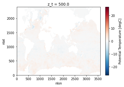
difference.isel(z_t=0).TEMP.plot()
<matplotlib.collections.QuadMesh at 0x2b1c89523a00>
Add a Helper Function to Make Sure the Colorbar is around 0#
def create_cmap(levs):
    """
    Creates a colormap using matplotlib.colors
    """
    assert len(levs) % 2 == 0, 'N levels must be even.'
    return colors.LinearSegmentedColormap.from_list(
        name='red_white_blue',
        colors=[(0, 0, 1), (1, 1.0, 1), (1, 0, 0)],
        N=len(levs) - 1,
    )


def generate_cbar(ds, var, lev=0):
    """
    Read in min/max values from a dataset and generate contour levels and a colorbar
    """
    ds = ds.isel(z_t=lev)
    max_diff = abs(np.nanmax(ds[var].values))
    min_diff = abs(np.nanmin(ds[var].values))
    max_diff = np.max(np.array(max_diff, min_diff))
    levels = list(np.linspace(-max_diff, max_diff, 20))
    cmap = create_cmap(levels)
    return levels, cmap
levels, cmap = generate_cbar(difference, 'TEMP')
difference.load()
difference.TEMP.hvplot.quadmesh(x='nlon', y='nlat', rasterize=True).opts(
    width=600, height=400, color_levels=levels, cmap=cmap, bgcolor='lightgray'
)
Conclusion#
In this example, we covered how useful xESMF can be when regridding between two different datasets. It is important to keep in mind the requirements for grid corner information when working with these different datasets.
In the future, this regridding step should be explored further in the context of applyin this at the time of data read in. For example, if one could add this step into the pangeo-forge recipe, the data access and preprocessing could be combined into a single step, enabling easier reproducibility and sharability.
This simplified, extensible workflow could be used to build a catalog of pre-gridded observations in a catalog similar to the example outlined in last week’s post, “Comparing Atmospheric Model Output with Observations Using Intake-ESM”