Processing Data from the NCAR Mesa Lab Weather Station

There is a weather station located at the Mesa Lab, situated along the Foothills of the Rockies in Boulder, Colorado!

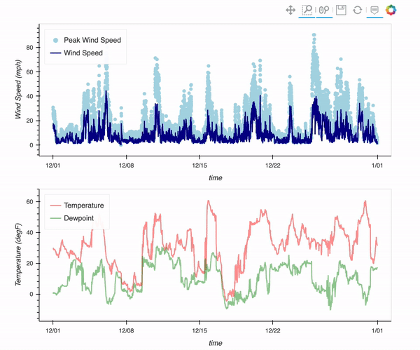
By the end of this post, you will be able to plot an interactive visualization of the weather data collected at the Mesa Lab, as shown below!

Here is a picture of the lab!

The Data

This station collects data every 10 minutes, is publicly available from this site, with live plots viewable here

For this example, we downloaded a month’s worth of daily data from December 2016. You can access the FTP server using this this link, pulling data from the /mesa directory. You will also need to unzip the files.

Imports

In this example, we utilize xarray and pandas for data cleaning, and hvplot/holoviews for visualization!

import holoviews as hv
import hvplot
import hvplot.xarray
import pandas as pd
import xarray as xr
from metpy.units import units

hv.extension('bokeh')

The Problem

When first accessing the data, you’ll notice that are file extenstions - .cdf and .nc

The data are all stored in netcdf format, which is a binary data format. If you are interested in learning more about netcdf, check out the Pythia Foundations material on “NetCDF and CF: The Basics”!

One issue here though is within the .cdf data… we can read in the data, but we do not have helpful time information…

We can load it in using xarray, as shown below!

cdf_ds = xr.open_dataset('mlab.20161201.cdf')
cdf_ds

<xarray.Dataset>
Dimensions:      (time: 288)
Dimensions without coordinates: time
Data variables: (12/20)
    base_time    int32 1480550400
    samp_secs    int32 300
    lat          float32 39.98
    lon          float32 -105.3
    alt          float32 1.885
    station      int32 0
    ...           ...
    wmax         (time) float32 13.8 13.0 11.2 11.6 11.3 ... 2.7 2.6 2.3 1.8 2.3
    wsdev        (time) float32 0.0 0.0 0.0 0.0 0.0 0.0 ... 0.0 0.0 0.0 0.0 0.0
    wchill       (time) float32 -14.4 -14.71 -13.76 -14.71 ... -0.6 -0.6 -0.6
    raina        (time) float32 0.0 0.0 0.0 0.0 0.0 0.0 ... 0.0 0.0 0.0 0.0 0.0
    raina24      (time) float32 0.0 0.0 0.0 0.0 0.0 0.0 ... 0.0 0.0 0.0 0.0 0.0
    bat          (time) float32 13.9 13.9 13.9 13.9 13.9 ... 13.9 13.9 13.9 13.9

Dealing with the time

We do have a few time related variables:

• base_time - number of seconds since 1970-01-01

• samp_secs - sample interval in seconds

• time_offset - number of seconds from base_time for a given observation

cdf_ds[['base_time', 'samp_secs', 'time_offset']]

<xarray.Dataset>
Dimensions:      (time: 288)
Dimensions without coordinates: time
Data variables:
    base_time    int32 1480550400
    samp_secs    int32 300
    time_offset  (time) float32 0.0 300.0 600.0 ... 8.55e+04 8.58e+04 8.61e+04

The Solution

Fortunately, we can use the time_offset variable, in conjunction with the base_time to determine a human-readable time dimension!

pandas.to_datetime has a helpful tool for this! If you are interested in learning more about this functionality, check out the official pandas.to_datetime documentation

Calculating the New Time Axis

We start first by calculating the time in units seconds since 1970-01-01, by adding the time_offset to base_time

new_time = cdf_ds.base_time + cdf_ds.time_offset
new_time

<xarray.DataArray (time: 288)>
array([1.4805504e+09, 1.4805507e+09, 1.4805510e+09, 1.4805513e+09,
       1.4805516e+09, 1.4805519e+09, 1.4805522e+09, 1.4805525e+09,
       1.4805528e+09, 1.4805531e+09, 1.4805534e+09, 1.4805537e+09,
       1.4805540e+09, 1.4805543e+09, 1.4805546e+09, 1.4805549e+09,
       1.4805552e+09, 1.4805555e+09, 1.4805558e+09, 1.4805561e+09,
       1.4805564e+09, 1.4805567e+09, 1.4805570e+09, 1.4805573e+09,
       1.4805576e+09, 1.4805579e+09, 1.4805582e+09, 1.4805585e+09,
       1.4805588e+09, 1.4805591e+09, 1.4805594e+09, 1.4805597e+09,
       1.4805600e+09, 1.4805603e+09, 1.4805606e+09, 1.4805609e+09,
       1.4805612e+09, 1.4805615e+09, 1.4805618e+09, 1.4805621e+09,
       1.4805624e+09, 1.4805627e+09, 1.4805630e+09, 1.4805633e+09,
       1.4805636e+09, 1.4805639e+09, 1.4805642e+09, 1.4805645e+09,
       1.4805648e+09, 1.4805651e+09, 1.4805654e+09, 1.4805657e+09,
       1.4805660e+09, 1.4805663e+09, 1.4805666e+09, 1.4805669e+09,
       1.4805672e+09, 1.4805675e+09, 1.4805678e+09, 1.4805681e+09,
       1.4805684e+09, 1.4805687e+09, 1.4805690e+09, 1.4805693e+09,
       1.4805696e+09, 1.4805699e+09, 1.4805702e+09, 1.4805705e+09,
       1.4805708e+09, 1.4805711e+09, 1.4805714e+09, 1.4805717e+09,
       1.4805720e+09, 1.4805723e+09, 1.4805726e+09, 1.4805729e+09,
       1.4805732e+09, 1.4805735e+09, 1.4805738e+09, 1.4805741e+09,
...
       1.4806128e+09, 1.4806131e+09, 1.4806134e+09, 1.4806137e+09,
       1.4806140e+09, 1.4806143e+09, 1.4806146e+09, 1.4806149e+09,
       1.4806152e+09, 1.4806155e+09, 1.4806158e+09, 1.4806161e+09,
       1.4806164e+09, 1.4806167e+09, 1.4806170e+09, 1.4806173e+09,
       1.4806176e+09, 1.4806179e+09, 1.4806182e+09, 1.4806185e+09,
       1.4806188e+09, 1.4806191e+09, 1.4806194e+09, 1.4806197e+09,
       1.4806200e+09, 1.4806203e+09, 1.4806206e+09, 1.4806209e+09,
       1.4806212e+09, 1.4806215e+09, 1.4806218e+09, 1.4806221e+09,
       1.4806224e+09, 1.4806227e+09, 1.4806230e+09, 1.4806233e+09,
       1.4806236e+09, 1.4806239e+09, 1.4806242e+09, 1.4806245e+09,
       1.4806248e+09, 1.4806251e+09, 1.4806254e+09, 1.4806257e+09,
       1.4806260e+09, 1.4806263e+09, 1.4806266e+09, 1.4806269e+09,
       1.4806272e+09, 1.4806275e+09, 1.4806278e+09, 1.4806281e+09,
       1.4806284e+09, 1.4806287e+09, 1.4806290e+09, 1.4806293e+09,
       1.4806296e+09, 1.4806299e+09, 1.4806302e+09, 1.4806305e+09,
       1.4806308e+09, 1.4806311e+09, 1.4806314e+09, 1.4806317e+09,
       1.4806320e+09, 1.4806323e+09, 1.4806326e+09, 1.4806329e+09,
       1.4806332e+09, 1.4806335e+09, 1.4806338e+09, 1.4806341e+09,
       1.4806344e+09, 1.4806347e+09, 1.4806350e+09, 1.4806353e+09,
       1.4806356e+09, 1.4806359e+09, 1.4806362e+09, 1.4806365e+09])
Dimensions without coordinates: time

That array is hard to read though… we can pass this into pandas.to_datetime to handle the conversion!

times = pd.to_datetime(new_time.values, unit='s')
times

DatetimeIndex(['2016-12-01 00:00:00', '2016-12-01 00:05:00',
               '2016-12-01 00:10:00', '2016-12-01 00:15:00',
               '2016-12-01 00:20:00', '2016-12-01 00:25:00',
               '2016-12-01 00:30:00', '2016-12-01 00:35:00',
               '2016-12-01 00:40:00', '2016-12-01 00:45:00',
               ...
               '2016-12-01 23:10:00', '2016-12-01 23:15:00',
               '2016-12-01 23:20:00', '2016-12-01 23:25:00',
               '2016-12-01 23:30:00', '2016-12-01 23:35:00',
               '2016-12-01 23:40:00', '2016-12-01 23:45:00',
               '2016-12-01 23:50:00', '2016-12-01 23:55:00'],
              dtype='datetime64[ns]', length=288, freq=None)

That looks better! We can now add this to our dimensions for the dataset.

cdf_ds['time'] = times
cdf_ds

<xarray.Dataset>
Dimensions:      (time: 288)
Coordinates:
  * time         (time) datetime64[ns] 2016-12-01 ... 2016-12-01T23:55:00
Data variables: (12/20)
    base_time    int32 1480550400
    samp_secs    int32 300
    lat          float32 39.98
    lon          float32 -105.3
    alt          float32 1.885
    station      int32 0
    ...           ...
    wmax         (time) float32 13.8 13.0 11.2 11.6 11.3 ... 2.7 2.6 2.3 1.8 2.3
    wsdev        (time) float32 0.0 0.0 0.0 0.0 0.0 0.0 ... 0.0 0.0 0.0 0.0 0.0
    wchill       (time) float32 -14.4 -14.71 -13.76 -14.71 ... -0.6 -0.6 -0.6
    raina        (time) float32 0.0 0.0 0.0 0.0 0.0 0.0 ... 0.0 0.0 0.0 0.0 0.0
    raina24      (time) float32 0.0 0.0 0.0 0.0 0.0 0.0 ... 0.0 0.0 0.0 0.0 0.0
    bat          (time) float32 13.9 13.9 13.9 13.9 13.9 ... 13.9 13.9 13.9 13.9

Wrapping into a Function and Using as a Preprocessor

We can wrap this into a function, then pass this into xr.open_mfdataset to process multiple files at the same time!

def fix_times(ds):
    ds['time'] = pd.to_datetime((ds.base_time + ds.time_offset).values, unit='s')
    return ds.drop(['base_time', 'samp_secs', 'time_offset'])

We can then pass our fix_time function into xr.open_mfdataset using the preprocess argument

ds = xr.open_mfdataset('*.cdf', engine='netcdf4', concat_dim='time', preprocess=fix_times).load()

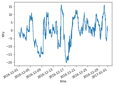
We can plot a basic plot using the .plot() method in xarray

ds.tdry.plot();

Plotting an Interactive Meteogram

We can also plot a “meteogram” which is a collection of different surface observations.

We know from the .nc files that variables have the following units:

• Temperature (tdry) - degrees Celsius

• Dewpoint (dp) - degrees Celsius

• Wind (wspd)- meter/second

• Max Wind Speed (wmax) - meter/second

We start by defining our plots, as shown below:

Converting to Standard Units

We can use metpy.units here to convert to US customary units!

ds_standard_units = ds.copy()

# Convert windspeed
ds_standard_units['wspd'] = ('time', (ds.wspd.values * units('m/s')).to('mph'))
ds_standard_units.wspd.attrs['units'] = 'mph'

# Convert max windspeed
ds_standard_units['wmax'] = ('time', (ds.wmax.values * units('m/s')).to('mph'))
ds_standard_units.wmax.attrs['units'] = 'mph'

# Convert windspeed
ds_standard_units['tdry'] = ('time', (ds.tdry.values * units('degC')).to('degF'))
ds_standard_units.tdry.attrs['units'] = 'degF'

# Convert max windspeed
ds_standard_units['dp'] = ('time', (ds.dp.values * units('degC')).to('degF'))
ds_standard_units.dp.attrs['units'] = 'degF'

Setup our Wind Plots

We now can setup our plots - starting with wind speed. We add a few labels, and merge them within the same subplot using the * syntax in holoviews!

wind_speed_plot = ds_standard_units.wspd.hvplot.line(
    ylabel='Wind Speed (mph)', color='darkblue', label='Wind Speed'
)
wind_speed_max_plot = ds_standard_units.wmax.hvplot.scatter(
    color='lightblue', label='Peak Wind Speed'
)
wind_speed_max_plot * wind_speed_plot

Setup our Temperature Plots

We follow the same process for our temperature/dewpoint plots, adding an alpha argument to lighten the colors a bit.

temperature_plot = ds_standard_units.tdry.hvplot.line(
    ylabel='Temperature (degF)', color='red', label='Temperature', alpha=0.4
)
dewpoint_plot = ds_standard_units.dp.hvplot.line(color='green', label='Dewpoint', alpha=0.4)
temperature_plot * dewpoint_plot

Bringing it All Together

Now that our plots are all setup, we can merge them into the same figure using the following syntax, specifying a single column and a legend located in the top left of each subplot:

hv.Layout(
    (wind_speed_max_plot * wind_speed_plot).opts(legend_position='top_left')
    + (temperature_plot * dewpoint_plot).opts(legend_position='top_left')
).cols(1)

Conclusion

Both Xarray and Pandas have helpful tools to deal with data cleaning, especially when working with time! Within this example, we showed how to apply this time cleaning step to data collected from the NCAR Mesa Lab Weather Station, passing this cleaning step into the preprocess argument in open_mfdataset!

Object Oriented Programming Tutorial   Correctly Calculating Annual Averages with Xarray