Correctly Calculating Annual Averages with Xarray#
A common component of people’s workflows is calculating annual averages, which helps reduce the frequency of datasets, making them easier to work with. Two of the data frequencies you may be looking to convert to annual include:
Daily (365 days in each year)
Monthly (12 months in a year)
The Data#
When using the daily data, calculating the averages is relatively straightforward since we do not have to do any weighting, taking the length of each time into account. We know that each day is equal in length, and there are 365 days in each year.
This is not the case with monthly data. When converting monthly frequency into annual frequency, we need to take the length of each month into account since not each month is created equal. For example, February has 28 days whereas December has 31 - we need to make sure to get the weights right.
In this example, we will be using monthly data from the CESM2-Large Ensemble which is stored on AWS.
The Problem#
Within Xarray, it can be tempting to use the resample or groupby functions to calculate your annual average, but you need to be careful here! By default these functions do not take the weight of the frequencies into account. We need to write a specialized workflow to account for this!
Here is a preview of how far off two different, seemingly similar methods of calculating annual averages with Xarray are!
The Solution#
Let’s dig into our solution - we will start by computing the yearly average from monthly data using resample, which is considered the “incorrect” method. Then, we will provide an example of calculating the proper weights, and applying these to our “correct” weighted average.
Imports#
We use some typical libraries (Xarray, Numpy, and Dask), along with some visualization packages (hvPlot and holoviews).
import holoviews as hv
import hvplot
import hvplot.xarray
import numpy as np
import xarray as xr
from distributed import Client
from ncar_jobqueue import NCARCluster
hv.extension('bokeh')


Spin up a Cluster#
We use our NCARCluster here and pass it to our Dask Client
cluster = NCARCluster()
cluster.scale(20)
client = Client(cluster)
client
/glade/work/mgrover/miniconda3/envs/cesm-collections-dev/lib/python3.9/site-packages/distributed/node.py:160: UserWarning: Port 8787 is already in use.
Perhaps you already have a cluster running?
Hosting the HTTP server on port 37603 instead
warnings.warn(
Client
Client-3747cfcf-4985-11ec-804b-3cecef1b11e4
| Connection method: Cluster object | Cluster type: dask_jobqueue.PBSCluster |
| Dashboard: https://jupyterhub.hpc.ucar.edu/stable/user/mgrover/proxy/37603/status |
Cluster Info
PBSCluster
39387129
| Dashboard: https://jupyterhub.hpc.ucar.edu/stable/user/mgrover/proxy/37603/status | Workers: 0 |
| Total threads: 0 | Total memory: 0 B |
Scheduler Info
Scheduler
Scheduler-7862b3d1-8869-44ba-bfe1-1cd0605d461b
| Comm: tcp://10.12.206.57:33692 | Workers: 0 |
| Dashboard: https://jupyterhub.hpc.ucar.edu/stable/user/mgrover/proxy/37603/status | Total threads: 0 |
| Started: Just now | Total memory: 0 B |
Workers
Load in the CESM2-LE Data#
We are using monthly potential temperature data from the CESM2 Large Ensemble. If you are interested in learning more about this dataset, check out the previous ESDS blog post looking at data from this ensemble.
ds = xr.open_zarr(
's3://ncar-cesm2-lens/ocn/monthly/cesm2LE-ssp370-cmip6-TEMP.zarr',
storage_options={'anon': True},
)
You’ll notice we have data from 2015 to 2100 - at monthly frequency! Let’s subset the first six years and first five ensemble members as a benchmark.
ds_first_five_years = ds.sel(time=slice('2015', '2019')).isel(member_id=range(5))
ds_first_five_years
<xarray.Dataset>
Dimensions: (member_id: 5, time: 60, z_t: 60, nlat: 384, nlon: 320, d2: 2)
Coordinates:
* member_id (member_id) <U12 'r10i1181p1f1' ... 'r10i1301p1f1'
* time (time) object 2015-01-16 12:00:00 ... 2019-12-16 12:00:00
time_bound (time, d2) object dask.array<chunksize=(60, 2), meta=np.ndarray>
* z_t (z_t) float32 500.0 1.5e+03 2.5e+03 ... 5.125e+05 5.375e+05
Dimensions without coordinates: nlat, nlon, d2
Data variables:
TEMP (member_id, time, z_t, nlat, nlon) float32 dask.array<chunksize=(1, 6, 60, 384, 320), meta=np.ndarray>
Attributes:
Conventions: CF-1.0; http://www.cgd.ucar.edu/cms/eaton/netcdf/CF-cu...
calendar: All years have exactly 365 days.
cell_methods: cell_methods = time: mean ==> the variable values are ...
contents: Diagnostic and Prognostic Variables
model_doi_url: https://doi.org/10.5065/D67H1H0V
revision: $Id$
source: CCSM POP2, the CCSM Ocean Component
time_period_freq: month_1- member_id: 5
- time: 60
- z_t: 60
- nlat: 384
- nlon: 320
- d2: 2
- member_id(member_id)<U12'r10i1181p1f1' ... 'r10i1301p1f1'
array(['r10i1181p1f1', 'r10i1231p1f1', 'r10i1251p1f1', 'r10i1281p1f1', 'r10i1301p1f1'], dtype='<U12') - time(time)object2015-01-16 12:00:00 ... 2019-12-...
- bounds :
- time_bound
- long_name :
- time
array([cftime.DatetimeNoLeap(2015, 1, 16, 12, 0, 0, 0, has_year_zero=True), cftime.DatetimeNoLeap(2015, 2, 15, 0, 0, 0, 0, has_year_zero=True), cftime.DatetimeNoLeap(2015, 3, 16, 12, 0, 0, 0, has_year_zero=True), cftime.DatetimeNoLeap(2015, 4, 16, 0, 0, 0, 0, has_year_zero=True), cftime.DatetimeNoLeap(2015, 5, 16, 12, 0, 0, 0, has_year_zero=True), cftime.DatetimeNoLeap(2015, 6, 16, 0, 0, 0, 0, has_year_zero=True), cftime.DatetimeNoLeap(2015, 7, 16, 12, 0, 0, 0, has_year_zero=True), cftime.DatetimeNoLeap(2015, 8, 16, 12, 0, 0, 0, has_year_zero=True), cftime.DatetimeNoLeap(2015, 9, 16, 0, 0, 0, 0, has_year_zero=True), cftime.DatetimeNoLeap(2015, 10, 16, 12, 0, 0, 0, has_year_zero=True), cftime.DatetimeNoLeap(2015, 11, 16, 0, 0, 0, 0, has_year_zero=True), cftime.DatetimeNoLeap(2015, 12, 16, 12, 0, 0, 0, has_year_zero=True), cftime.DatetimeNoLeap(2016, 1, 16, 12, 0, 0, 0, has_year_zero=True), cftime.DatetimeNoLeap(2016, 2, 15, 0, 0, 0, 0, has_year_zero=True), cftime.DatetimeNoLeap(2016, 3, 16, 12, 0, 0, 0, has_year_zero=True), cftime.DatetimeNoLeap(2016, 4, 16, 0, 0, 0, 0, has_year_zero=True), cftime.DatetimeNoLeap(2016, 5, 16, 12, 0, 0, 0, has_year_zero=True), cftime.DatetimeNoLeap(2016, 6, 16, 0, 0, 0, 0, has_year_zero=True), cftime.DatetimeNoLeap(2016, 7, 16, 12, 0, 0, 0, has_year_zero=True), cftime.DatetimeNoLeap(2016, 8, 16, 12, 0, 0, 0, has_year_zero=True), cftime.DatetimeNoLeap(2016, 9, 16, 0, 0, 0, 0, has_year_zero=True), cftime.DatetimeNoLeap(2016, 10, 16, 12, 0, 0, 0, has_year_zero=True), cftime.DatetimeNoLeap(2016, 11, 16, 0, 0, 0, 0, has_year_zero=True), cftime.DatetimeNoLeap(2016, 12, 16, 12, 0, 0, 0, has_year_zero=True), cftime.DatetimeNoLeap(2017, 1, 16, 12, 0, 0, 0, has_year_zero=True), cftime.DatetimeNoLeap(2017, 2, 15, 0, 0, 0, 0, has_year_zero=True), cftime.DatetimeNoLeap(2017, 3, 16, 12, 0, 0, 0, has_year_zero=True), cftime.DatetimeNoLeap(2017, 4, 16, 0, 0, 0, 0, has_year_zero=True), cftime.DatetimeNoLeap(2017, 5, 16, 12, 0, 0, 0, has_year_zero=True), cftime.DatetimeNoLeap(2017, 6, 16, 0, 0, 0, 0, has_year_zero=True), cftime.DatetimeNoLeap(2017, 7, 16, 12, 0, 0, 0, has_year_zero=True), cftime.DatetimeNoLeap(2017, 8, 16, 12, 0, 0, 0, has_year_zero=True), cftime.DatetimeNoLeap(2017, 9, 16, 0, 0, 0, 0, has_year_zero=True), cftime.DatetimeNoLeap(2017, 10, 16, 12, 0, 0, 0, has_year_zero=True), cftime.DatetimeNoLeap(2017, 11, 16, 0, 0, 0, 0, has_year_zero=True), cftime.DatetimeNoLeap(2017, 12, 16, 12, 0, 0, 0, has_year_zero=True), cftime.DatetimeNoLeap(2018, 1, 16, 12, 0, 0, 0, has_year_zero=True), cftime.DatetimeNoLeap(2018, 2, 15, 0, 0, 0, 0, has_year_zero=True), cftime.DatetimeNoLeap(2018, 3, 16, 12, 0, 0, 0, has_year_zero=True), cftime.DatetimeNoLeap(2018, 4, 16, 0, 0, 0, 0, has_year_zero=True), cftime.DatetimeNoLeap(2018, 5, 16, 12, 0, 0, 0, has_year_zero=True), cftime.DatetimeNoLeap(2018, 6, 16, 0, 0, 0, 0, has_year_zero=True), cftime.DatetimeNoLeap(2018, 7, 16, 12, 0, 0, 0, has_year_zero=True), cftime.DatetimeNoLeap(2018, 8, 16, 12, 0, 0, 0, has_year_zero=True), cftime.DatetimeNoLeap(2018, 9, 16, 0, 0, 0, 0, has_year_zero=True), cftime.DatetimeNoLeap(2018, 10, 16, 12, 0, 0, 0, has_year_zero=True), cftime.DatetimeNoLeap(2018, 11, 16, 0, 0, 0, 0, has_year_zero=True), cftime.DatetimeNoLeap(2018, 12, 16, 12, 0, 0, 0, has_year_zero=True), cftime.DatetimeNoLeap(2019, 1, 16, 12, 0, 0, 0, has_year_zero=True), cftime.DatetimeNoLeap(2019, 2, 15, 0, 0, 0, 0, has_year_zero=True), cftime.DatetimeNoLeap(2019, 3, 16, 12, 0, 0, 0, has_year_zero=True), cftime.DatetimeNoLeap(2019, 4, 16, 0, 0, 0, 0, has_year_zero=True), cftime.DatetimeNoLeap(2019, 5, 16, 12, 0, 0, 0, has_year_zero=True), cftime.DatetimeNoLeap(2019, 6, 16, 0, 0, 0, 0, has_year_zero=True), cftime.DatetimeNoLeap(2019, 7, 16, 12, 0, 0, 0, has_year_zero=True), cftime.DatetimeNoLeap(2019, 8, 16, 12, 0, 0, 0, has_year_zero=True), cftime.DatetimeNoLeap(2019, 9, 16, 0, 0, 0, 0, has_year_zero=True), cftime.DatetimeNoLeap(2019, 10, 16, 12, 0, 0, 0, has_year_zero=True), cftime.DatetimeNoLeap(2019, 11, 16, 0, 0, 0, 0, has_year_zero=True), cftime.DatetimeNoLeap(2019, 12, 16, 12, 0, 0, 0, has_year_zero=True)], dtype=object) - time_bound(time, d2)objectdask.array<chunksize=(60, 2), meta=np.ndarray>
- long_name :
- boundaries for time-averaging interval
Array Chunk Bytes 0.94 kiB 0.94 kiB Shape (60, 2) (60, 2) Count 3 Tasks 1 Chunks Type object numpy.ndarray - z_t(z_t)float32500.0 1.5e+03 ... 5.375e+05
- long_name :
- depth from surface to midpoint of layer
- positive :
- down
- units :
- centimeters
- valid_max :
- 537500.0
- valid_min :
- 500.0
array([5.000000e+02, 1.500000e+03, 2.500000e+03, 3.500000e+03, 4.500000e+03, 5.500000e+03, 6.500000e+03, 7.500000e+03, 8.500000e+03, 9.500000e+03, 1.050000e+04, 1.150000e+04, 1.250000e+04, 1.350000e+04, 1.450000e+04, 1.550000e+04, 1.650984e+04, 1.754790e+04, 1.862913e+04, 1.976603e+04, 2.097114e+04, 2.225783e+04, 2.364088e+04, 2.513702e+04, 2.676542e+04, 2.854837e+04, 3.051192e+04, 3.268680e+04, 3.510935e+04, 3.782276e+04, 4.087846e+04, 4.433777e+04, 4.827367e+04, 5.277280e+04, 5.793729e+04, 6.388626e+04, 7.075633e+04, 7.870025e+04, 8.788252e+04, 9.847059e+04, 1.106204e+05, 1.244567e+05, 1.400497e+05, 1.573946e+05, 1.764003e+05, 1.968944e+05, 2.186457e+05, 2.413972e+05, 2.649001e+05, 2.889385e+05, 3.133405e+05, 3.379793e+05, 3.627670e+05, 3.876452e+05, 4.125768e+05, 4.375392e+05, 4.625190e+05, 4.875083e+05, 5.125028e+05, 5.375000e+05], dtype=float32)
- TEMP(member_id, time, z_t, nlat, nlon)float32dask.array<chunksize=(1, 6, 60, 384, 320), meta=np.ndarray>
- cell_methods :
- time: mean
- coordinates :
- TLONG TLAT z_t time
- grid_loc :
- 3111
- long_name :
- Potential Temperature
- units :
- degC
Array Chunk Bytes 8.24 GiB 168.75 MiB Shape (5, 60, 60, 384, 320) (1, 6, 60, 384, 320) Count 9151 Tasks 50 Chunks Type float32 numpy.ndarray
- Conventions :
- CF-1.0; http://www.cgd.ucar.edu/cms/eaton/netcdf/CF-current.htm
- calendar :
- All years have exactly 365 days.
- cell_methods :
- cell_methods = time: mean ==> the variable values are averaged over the time interval between the previous time coordinate and the current one. cell_methods absent ==> the variable values are at the time given by the current time coordinate.
- contents :
- Diagnostic and Prognostic Variables
- model_doi_url :
- https://doi.org/10.5065/D67H1H0V
- revision :
- $Id$
- source :
- CCSM POP2, the CCSM Ocean Component
- time_period_freq :
- month_1
Calculate the Annual Average Incorrectly#
We can try using resample here to calculate the annual average, from a subset of the data
The resample method comes from Pandas! If you are interested in learning more about this functionality, check out their docs
The frequency we are looking for is AS, which is the annual frequency.
We can calculate our resampled dataset using the following
resampled = ds_first_five_years.resample(time='AS').mean('time')
This will lazily calculate the data - in order to check to see how long this takes, we can add the %%time magic command at the top of the cell
%%time
yearly_average_weighted_incorrectly = resampled.compute()
CPU times: user 970 ms, sys: 1.28 s, total: 2.25 s
Wall time: 19.8 s
Let’s get a quick plot of the data!
yearly_average_weighted_incorrectly.TEMP.isel(z_t=0, nlat=100, nlon=100).plot(x='time');
/glade/work/mgrover/miniconda3/envs/cesm-collections-dev/lib/python3.9/site-packages/xarray/plot/plot.py:1476: MatplotlibDeprecationWarning: shading='flat' when X and Y have the same dimensions as C is deprecated since 3.3. Either specify the corners of the quadrilaterals with X and Y, or pass shading='auto', 'nearest' or 'gouraud', or set rcParams['pcolor.shading']. This will become an error two minor releases later.
primitive = ax.pcolormesh(x, y, z, **kwargs)
Calculating the Yearly Average Correctly#
As mentioned previously, we need to weight the months correctly. We can do this by determining how many days are in each month.
We can use the .dt method on the times in our dataset to extract the number of days in each month! Which can be super helpful 👍
month_length = ds_first_five_years.time.dt.days_in_month
month_length
<xarray.DataArray 'days_in_month' (time: 60)>
array([31, 28, 31, 30, 31, 30, 31, 31, 30, 31, 30, 31, 31, 28, 31, 30, 31,
30, 31, 31, 30, 31, 30, 31, 31, 28, 31, 30, 31, 30, 31, 31, 30, 31,
30, 31, 31, 28, 31, 30, 31, 30, 31, 31, 30, 31, 30, 31, 31, 28, 31,
30, 31, 30, 31, 31, 30, 31, 30, 31])
Coordinates:
* time (time) object 2015-01-16 12:00:00 ... 2019-12-16 12:00:00- time: 60
- 31 28 31 30 31 30 31 31 30 31 30 ... 28 31 30 31 30 31 31 30 31 30 31
array([31, 28, 31, 30, 31, 30, 31, 31, 30, 31, 30, 31, 31, 28, 31, 30, 31, 30, 31, 31, 30, 31, 30, 31, 31, 28, 31, 30, 31, 30, 31, 31, 30, 31, 30, 31, 31, 28, 31, 30, 31, 30, 31, 31, 30, 31, 30, 31, 31, 28, 31, 30, 31, 30, 31, 31, 30, 31, 30, 31]) - time(time)object2015-01-16 12:00:00 ... 2019-12-...
- bounds :
- time_bound
- long_name :
- time
array([cftime.DatetimeNoLeap(2015, 1, 16, 12, 0, 0, 0, has_year_zero=True), cftime.DatetimeNoLeap(2015, 2, 15, 0, 0, 0, 0, has_year_zero=True), cftime.DatetimeNoLeap(2015, 3, 16, 12, 0, 0, 0, has_year_zero=True), cftime.DatetimeNoLeap(2015, 4, 16, 0, 0, 0, 0, has_year_zero=True), cftime.DatetimeNoLeap(2015, 5, 16, 12, 0, 0, 0, has_year_zero=True), cftime.DatetimeNoLeap(2015, 6, 16, 0, 0, 0, 0, has_year_zero=True), cftime.DatetimeNoLeap(2015, 7, 16, 12, 0, 0, 0, has_year_zero=True), cftime.DatetimeNoLeap(2015, 8, 16, 12, 0, 0, 0, has_year_zero=True), cftime.DatetimeNoLeap(2015, 9, 16, 0, 0, 0, 0, has_year_zero=True), cftime.DatetimeNoLeap(2015, 10, 16, 12, 0, 0, 0, has_year_zero=True), cftime.DatetimeNoLeap(2015, 11, 16, 0, 0, 0, 0, has_year_zero=True), cftime.DatetimeNoLeap(2015, 12, 16, 12, 0, 0, 0, has_year_zero=True), cftime.DatetimeNoLeap(2016, 1, 16, 12, 0, 0, 0, has_year_zero=True), cftime.DatetimeNoLeap(2016, 2, 15, 0, 0, 0, 0, has_year_zero=True), cftime.DatetimeNoLeap(2016, 3, 16, 12, 0, 0, 0, has_year_zero=True), cftime.DatetimeNoLeap(2016, 4, 16, 0, 0, 0, 0, has_year_zero=True), cftime.DatetimeNoLeap(2016, 5, 16, 12, 0, 0, 0, has_year_zero=True), cftime.DatetimeNoLeap(2016, 6, 16, 0, 0, 0, 0, has_year_zero=True), cftime.DatetimeNoLeap(2016, 7, 16, 12, 0, 0, 0, has_year_zero=True), cftime.DatetimeNoLeap(2016, 8, 16, 12, 0, 0, 0, has_year_zero=True), cftime.DatetimeNoLeap(2016, 9, 16, 0, 0, 0, 0, has_year_zero=True), cftime.DatetimeNoLeap(2016, 10, 16, 12, 0, 0, 0, has_year_zero=True), cftime.DatetimeNoLeap(2016, 11, 16, 0, 0, 0, 0, has_year_zero=True), cftime.DatetimeNoLeap(2016, 12, 16, 12, 0, 0, 0, has_year_zero=True), cftime.DatetimeNoLeap(2017, 1, 16, 12, 0, 0, 0, has_year_zero=True), cftime.DatetimeNoLeap(2017, 2, 15, 0, 0, 0, 0, has_year_zero=True), cftime.DatetimeNoLeap(2017, 3, 16, 12, 0, 0, 0, has_year_zero=True), cftime.DatetimeNoLeap(2017, 4, 16, 0, 0, 0, 0, has_year_zero=True), cftime.DatetimeNoLeap(2017, 5, 16, 12, 0, 0, 0, has_year_zero=True), cftime.DatetimeNoLeap(2017, 6, 16, 0, 0, 0, 0, has_year_zero=True), cftime.DatetimeNoLeap(2017, 7, 16, 12, 0, 0, 0, has_year_zero=True), cftime.DatetimeNoLeap(2017, 8, 16, 12, 0, 0, 0, has_year_zero=True), cftime.DatetimeNoLeap(2017, 9, 16, 0, 0, 0, 0, has_year_zero=True), cftime.DatetimeNoLeap(2017, 10, 16, 12, 0, 0, 0, has_year_zero=True), cftime.DatetimeNoLeap(2017, 11, 16, 0, 0, 0, 0, has_year_zero=True), cftime.DatetimeNoLeap(2017, 12, 16, 12, 0, 0, 0, has_year_zero=True), cftime.DatetimeNoLeap(2018, 1, 16, 12, 0, 0, 0, has_year_zero=True), cftime.DatetimeNoLeap(2018, 2, 15, 0, 0, 0, 0, has_year_zero=True), cftime.DatetimeNoLeap(2018, 3, 16, 12, 0, 0, 0, has_year_zero=True), cftime.DatetimeNoLeap(2018, 4, 16, 0, 0, 0, 0, has_year_zero=True), cftime.DatetimeNoLeap(2018, 5, 16, 12, 0, 0, 0, has_year_zero=True), cftime.DatetimeNoLeap(2018, 6, 16, 0, 0, 0, 0, has_year_zero=True), cftime.DatetimeNoLeap(2018, 7, 16, 12, 0, 0, 0, has_year_zero=True), cftime.DatetimeNoLeap(2018, 8, 16, 12, 0, 0, 0, has_year_zero=True), cftime.DatetimeNoLeap(2018, 9, 16, 0, 0, 0, 0, has_year_zero=True), cftime.DatetimeNoLeap(2018, 10, 16, 12, 0, 0, 0, has_year_zero=True), cftime.DatetimeNoLeap(2018, 11, 16, 0, 0, 0, 0, has_year_zero=True), cftime.DatetimeNoLeap(2018, 12, 16, 12, 0, 0, 0, has_year_zero=True), cftime.DatetimeNoLeap(2019, 1, 16, 12, 0, 0, 0, has_year_zero=True), cftime.DatetimeNoLeap(2019, 2, 15, 0, 0, 0, 0, has_year_zero=True), cftime.DatetimeNoLeap(2019, 3, 16, 12, 0, 0, 0, has_year_zero=True), cftime.DatetimeNoLeap(2019, 4, 16, 0, 0, 0, 0, has_year_zero=True), cftime.DatetimeNoLeap(2019, 5, 16, 12, 0, 0, 0, has_year_zero=True), cftime.DatetimeNoLeap(2019, 6, 16, 0, 0, 0, 0, has_year_zero=True), cftime.DatetimeNoLeap(2019, 7, 16, 12, 0, 0, 0, has_year_zero=True), cftime.DatetimeNoLeap(2019, 8, 16, 12, 0, 0, 0, has_year_zero=True), cftime.DatetimeNoLeap(2019, 9, 16, 0, 0, 0, 0, has_year_zero=True), cftime.DatetimeNoLeap(2019, 10, 16, 12, 0, 0, 0, has_year_zero=True), cftime.DatetimeNoLeap(2019, 11, 16, 0, 0, 0, 0, has_year_zero=True), cftime.DatetimeNoLeap(2019, 12, 16, 12, 0, 0, 0, has_year_zero=True)], dtype=object)
We can calculate our weights using the following, which results in an xarray.DataArray with the corresponding weights.
Notice how longer months (ex. months with 31 days) have a higher weight than months with less days (ex. 28)
wgts = month_length.groupby("time.year") / month_length.groupby("time.year").sum()
wgts
<xarray.DataArray 'days_in_month' (time: 60)>
array([0.08493151, 0.07671233, 0.08493151, 0.08219178, 0.08493151,
0.08219178, 0.08493151, 0.08493151, 0.08219178, 0.08493151,
0.08219178, 0.08493151, 0.08493151, 0.07671233, 0.08493151,
0.08219178, 0.08493151, 0.08219178, 0.08493151, 0.08493151,
0.08219178, 0.08493151, 0.08219178, 0.08493151, 0.08493151,
0.07671233, 0.08493151, 0.08219178, 0.08493151, 0.08219178,
0.08493151, 0.08493151, 0.08219178, 0.08493151, 0.08219178,
0.08493151, 0.08493151, 0.07671233, 0.08493151, 0.08219178,
0.08493151, 0.08219178, 0.08493151, 0.08493151, 0.08219178,
0.08493151, 0.08219178, 0.08493151, 0.08493151, 0.07671233,
0.08493151, 0.08219178, 0.08493151, 0.08219178, 0.08493151,
0.08493151, 0.08219178, 0.08493151, 0.08219178, 0.08493151])
Coordinates:
* time (time) object 2015-01-16 12:00:00 ... 2019-12-16 12:00:00
year (time) int64 2015 2015 2015 2015 2015 ... 2019 2019 2019 2019 2019- time: 60
- 0.08493 0.07671 0.08493 0.08219 ... 0.08219 0.08493 0.08219 0.08493
array([0.08493151, 0.07671233, 0.08493151, 0.08219178, 0.08493151, 0.08219178, 0.08493151, 0.08493151, 0.08219178, 0.08493151, 0.08219178, 0.08493151, 0.08493151, 0.07671233, 0.08493151, 0.08219178, 0.08493151, 0.08219178, 0.08493151, 0.08493151, 0.08219178, 0.08493151, 0.08219178, 0.08493151, 0.08493151, 0.07671233, 0.08493151, 0.08219178, 0.08493151, 0.08219178, 0.08493151, 0.08493151, 0.08219178, 0.08493151, 0.08219178, 0.08493151, 0.08493151, 0.07671233, 0.08493151, 0.08219178, 0.08493151, 0.08219178, 0.08493151, 0.08493151, 0.08219178, 0.08493151, 0.08219178, 0.08493151, 0.08493151, 0.07671233, 0.08493151, 0.08219178, 0.08493151, 0.08219178, 0.08493151, 0.08493151, 0.08219178, 0.08493151, 0.08219178, 0.08493151]) - time(time)object2015-01-16 12:00:00 ... 2019-12-...
- bounds :
- time_bound
- long_name :
- time
array([cftime.DatetimeNoLeap(2015, 1, 16, 12, 0, 0, 0, has_year_zero=True), cftime.DatetimeNoLeap(2015, 2, 15, 0, 0, 0, 0, has_year_zero=True), cftime.DatetimeNoLeap(2015, 3, 16, 12, 0, 0, 0, has_year_zero=True), cftime.DatetimeNoLeap(2015, 4, 16, 0, 0, 0, 0, has_year_zero=True), cftime.DatetimeNoLeap(2015, 5, 16, 12, 0, 0, 0, has_year_zero=True), cftime.DatetimeNoLeap(2015, 6, 16, 0, 0, 0, 0, has_year_zero=True), cftime.DatetimeNoLeap(2015, 7, 16, 12, 0, 0, 0, has_year_zero=True), cftime.DatetimeNoLeap(2015, 8, 16, 12, 0, 0, 0, has_year_zero=True), cftime.DatetimeNoLeap(2015, 9, 16, 0, 0, 0, 0, has_year_zero=True), cftime.DatetimeNoLeap(2015, 10, 16, 12, 0, 0, 0, has_year_zero=True), cftime.DatetimeNoLeap(2015, 11, 16, 0, 0, 0, 0, has_year_zero=True), cftime.DatetimeNoLeap(2015, 12, 16, 12, 0, 0, 0, has_year_zero=True), cftime.DatetimeNoLeap(2016, 1, 16, 12, 0, 0, 0, has_year_zero=True), cftime.DatetimeNoLeap(2016, 2, 15, 0, 0, 0, 0, has_year_zero=True), cftime.DatetimeNoLeap(2016, 3, 16, 12, 0, 0, 0, has_year_zero=True), cftime.DatetimeNoLeap(2016, 4, 16, 0, 0, 0, 0, has_year_zero=True), cftime.DatetimeNoLeap(2016, 5, 16, 12, 0, 0, 0, has_year_zero=True), cftime.DatetimeNoLeap(2016, 6, 16, 0, 0, 0, 0, has_year_zero=True), cftime.DatetimeNoLeap(2016, 7, 16, 12, 0, 0, 0, has_year_zero=True), cftime.DatetimeNoLeap(2016, 8, 16, 12, 0, 0, 0, has_year_zero=True), cftime.DatetimeNoLeap(2016, 9, 16, 0, 0, 0, 0, has_year_zero=True), cftime.DatetimeNoLeap(2016, 10, 16, 12, 0, 0, 0, has_year_zero=True), cftime.DatetimeNoLeap(2016, 11, 16, 0, 0, 0, 0, has_year_zero=True), cftime.DatetimeNoLeap(2016, 12, 16, 12, 0, 0, 0, has_year_zero=True), cftime.DatetimeNoLeap(2017, 1, 16, 12, 0, 0, 0, has_year_zero=True), cftime.DatetimeNoLeap(2017, 2, 15, 0, 0, 0, 0, has_year_zero=True), cftime.DatetimeNoLeap(2017, 3, 16, 12, 0, 0, 0, has_year_zero=True), cftime.DatetimeNoLeap(2017, 4, 16, 0, 0, 0, 0, has_year_zero=True), cftime.DatetimeNoLeap(2017, 5, 16, 12, 0, 0, 0, has_year_zero=True), cftime.DatetimeNoLeap(2017, 6, 16, 0, 0, 0, 0, has_year_zero=True), cftime.DatetimeNoLeap(2017, 7, 16, 12, 0, 0, 0, has_year_zero=True), cftime.DatetimeNoLeap(2017, 8, 16, 12, 0, 0, 0, has_year_zero=True), cftime.DatetimeNoLeap(2017, 9, 16, 0, 0, 0, 0, has_year_zero=True), cftime.DatetimeNoLeap(2017, 10, 16, 12, 0, 0, 0, has_year_zero=True), cftime.DatetimeNoLeap(2017, 11, 16, 0, 0, 0, 0, has_year_zero=True), cftime.DatetimeNoLeap(2017, 12, 16, 12, 0, 0, 0, has_year_zero=True), cftime.DatetimeNoLeap(2018, 1, 16, 12, 0, 0, 0, has_year_zero=True), cftime.DatetimeNoLeap(2018, 2, 15, 0, 0, 0, 0, has_year_zero=True), cftime.DatetimeNoLeap(2018, 3, 16, 12, 0, 0, 0, has_year_zero=True), cftime.DatetimeNoLeap(2018, 4, 16, 0, 0, 0, 0, has_year_zero=True), cftime.DatetimeNoLeap(2018, 5, 16, 12, 0, 0, 0, has_year_zero=True), cftime.DatetimeNoLeap(2018, 6, 16, 0, 0, 0, 0, has_year_zero=True), cftime.DatetimeNoLeap(2018, 7, 16, 12, 0, 0, 0, has_year_zero=True), cftime.DatetimeNoLeap(2018, 8, 16, 12, 0, 0, 0, has_year_zero=True), cftime.DatetimeNoLeap(2018, 9, 16, 0, 0, 0, 0, has_year_zero=True), cftime.DatetimeNoLeap(2018, 10, 16, 12, 0, 0, 0, has_year_zero=True), cftime.DatetimeNoLeap(2018, 11, 16, 0, 0, 0, 0, has_year_zero=True), cftime.DatetimeNoLeap(2018, 12, 16, 12, 0, 0, 0, has_year_zero=True), cftime.DatetimeNoLeap(2019, 1, 16, 12, 0, 0, 0, has_year_zero=True), cftime.DatetimeNoLeap(2019, 2, 15, 0, 0, 0, 0, has_year_zero=True), cftime.DatetimeNoLeap(2019, 3, 16, 12, 0, 0, 0, has_year_zero=True), cftime.DatetimeNoLeap(2019, 4, 16, 0, 0, 0, 0, has_year_zero=True), cftime.DatetimeNoLeap(2019, 5, 16, 12, 0, 0, 0, has_year_zero=True), cftime.DatetimeNoLeap(2019, 6, 16, 0, 0, 0, 0, has_year_zero=True), cftime.DatetimeNoLeap(2019, 7, 16, 12, 0, 0, 0, has_year_zero=True), cftime.DatetimeNoLeap(2019, 8, 16, 12, 0, 0, 0, has_year_zero=True), cftime.DatetimeNoLeap(2019, 9, 16, 0, 0, 0, 0, has_year_zero=True), cftime.DatetimeNoLeap(2019, 10, 16, 12, 0, 0, 0, has_year_zero=True), cftime.DatetimeNoLeap(2019, 11, 16, 0, 0, 0, 0, has_year_zero=True), cftime.DatetimeNoLeap(2019, 12, 16, 12, 0, 0, 0, has_year_zero=True)], dtype=object) - year(time)int642015 2015 2015 ... 2019 2019 2019
array([2015, 2015, 2015, 2015, 2015, 2015, 2015, 2015, 2015, 2015, 2015, 2015, 2016, 2016, 2016, 2016, 2016, 2016, 2016, 2016, 2016, 2016, 2016, 2016, 2017, 2017, 2017, 2017, 2017, 2017, 2017, 2017, 2017, 2017, 2017, 2017, 2018, 2018, 2018, 2018, 2018, 2018, 2018, 2018, 2018, 2018, 2018, 2018, 2019, 2019, 2019, 2019, 2019, 2019, 2019, 2019, 2019, 2019, 2019, 2019])
We should run a test to make sure that all these weights add up to 1, which can be accomplished using a helpful numpy.testing function.
This is making sure that sum of each year’s weights is equal to 1!
np.testing.assert_allclose(wgts.groupby("time.year").sum(xr.ALL_DIMS), 1.0)
We could just print out the sum to take a look too
wgts.groupby("time.year").sum(xr.ALL_DIMS)
<xarray.DataArray 'days_in_month' (year: 5)> array([1., 1., 1., 1., 1.]) Coordinates: * year (year) int64 2015 2016 2017 2018 2019
- year: 5
- 1.0 1.0 1.0 1.0 1.0
array([1., 1., 1., 1., 1.])
- year(year)int642015 2016 2017 2018 2019
array([2015, 2016, 2017, 2018, 2019])
Now that we have our weights, we need to apply them to our dataset. We can still use resample here too!
temp = ds_first_five_years['TEMP']
temp
<xarray.DataArray 'TEMP' (member_id: 5, time: 60, z_t: 60, nlat: 384, nlon: 320)>
dask.array<getitem, shape=(5, 60, 60, 384, 320), dtype=float32, chunksize=(1, 6, 60, 384, 320), chunktype=numpy.ndarray>
Coordinates:
* member_id (member_id) <U12 'r10i1181p1f1' 'r10i1231p1f1' ... 'r10i1301p1f1'
* time (time) object 2015-01-16 12:00:00 ... 2019-12-16 12:00:00
* z_t (z_t) float32 500.0 1.5e+03 2.5e+03 ... 5.125e+05 5.375e+05
Dimensions without coordinates: nlat, nlon
Attributes:
cell_methods: time: mean
coordinates: TLONG TLAT z_t time
grid_loc: 3111
long_name: Potential Temperature
units: degC- member_id: 5
- time: 60
- z_t: 60
- nlat: 384
- nlon: 320
- dask.array<chunksize=(1, 6, 60, 384, 320), meta=np.ndarray>
Array Chunk Bytes 8.24 GiB 168.75 MiB Shape (5, 60, 60, 384, 320) (1, 6, 60, 384, 320) Count 9151 Tasks 50 Chunks Type float32 numpy.ndarray - member_id(member_id)<U12'r10i1181p1f1' ... 'r10i1301p1f1'
array(['r10i1181p1f1', 'r10i1231p1f1', 'r10i1251p1f1', 'r10i1281p1f1', 'r10i1301p1f1'], dtype='<U12') - time(time)object2015-01-16 12:00:00 ... 2019-12-...
- bounds :
- time_bound
- long_name :
- time
array([cftime.DatetimeNoLeap(2015, 1, 16, 12, 0, 0, 0, has_year_zero=True), cftime.DatetimeNoLeap(2015, 2, 15, 0, 0, 0, 0, has_year_zero=True), cftime.DatetimeNoLeap(2015, 3, 16, 12, 0, 0, 0, has_year_zero=True), cftime.DatetimeNoLeap(2015, 4, 16, 0, 0, 0, 0, has_year_zero=True), cftime.DatetimeNoLeap(2015, 5, 16, 12, 0, 0, 0, has_year_zero=True), cftime.DatetimeNoLeap(2015, 6, 16, 0, 0, 0, 0, has_year_zero=True), cftime.DatetimeNoLeap(2015, 7, 16, 12, 0, 0, 0, has_year_zero=True), cftime.DatetimeNoLeap(2015, 8, 16, 12, 0, 0, 0, has_year_zero=True), cftime.DatetimeNoLeap(2015, 9, 16, 0, 0, 0, 0, has_year_zero=True), cftime.DatetimeNoLeap(2015, 10, 16, 12, 0, 0, 0, has_year_zero=True), cftime.DatetimeNoLeap(2015, 11, 16, 0, 0, 0, 0, has_year_zero=True), cftime.DatetimeNoLeap(2015, 12, 16, 12, 0, 0, 0, has_year_zero=True), cftime.DatetimeNoLeap(2016, 1, 16, 12, 0, 0, 0, has_year_zero=True), cftime.DatetimeNoLeap(2016, 2, 15, 0, 0, 0, 0, has_year_zero=True), cftime.DatetimeNoLeap(2016, 3, 16, 12, 0, 0, 0, has_year_zero=True), cftime.DatetimeNoLeap(2016, 4, 16, 0, 0, 0, 0, has_year_zero=True), cftime.DatetimeNoLeap(2016, 5, 16, 12, 0, 0, 0, has_year_zero=True), cftime.DatetimeNoLeap(2016, 6, 16, 0, 0, 0, 0, has_year_zero=True), cftime.DatetimeNoLeap(2016, 7, 16, 12, 0, 0, 0, has_year_zero=True), cftime.DatetimeNoLeap(2016, 8, 16, 12, 0, 0, 0, has_year_zero=True), cftime.DatetimeNoLeap(2016, 9, 16, 0, 0, 0, 0, has_year_zero=True), cftime.DatetimeNoLeap(2016, 10, 16, 12, 0, 0, 0, has_year_zero=True), cftime.DatetimeNoLeap(2016, 11, 16, 0, 0, 0, 0, has_year_zero=True), cftime.DatetimeNoLeap(2016, 12, 16, 12, 0, 0, 0, has_year_zero=True), cftime.DatetimeNoLeap(2017, 1, 16, 12, 0, 0, 0, has_year_zero=True), cftime.DatetimeNoLeap(2017, 2, 15, 0, 0, 0, 0, has_year_zero=True), cftime.DatetimeNoLeap(2017, 3, 16, 12, 0, 0, 0, has_year_zero=True), cftime.DatetimeNoLeap(2017, 4, 16, 0, 0, 0, 0, has_year_zero=True), cftime.DatetimeNoLeap(2017, 5, 16, 12, 0, 0, 0, has_year_zero=True), cftime.DatetimeNoLeap(2017, 6, 16, 0, 0, 0, 0, has_year_zero=True), cftime.DatetimeNoLeap(2017, 7, 16, 12, 0, 0, 0, has_year_zero=True), cftime.DatetimeNoLeap(2017, 8, 16, 12, 0, 0, 0, has_year_zero=True), cftime.DatetimeNoLeap(2017, 9, 16, 0, 0, 0, 0, has_year_zero=True), cftime.DatetimeNoLeap(2017, 10, 16, 12, 0, 0, 0, has_year_zero=True), cftime.DatetimeNoLeap(2017, 11, 16, 0, 0, 0, 0, has_year_zero=True), cftime.DatetimeNoLeap(2017, 12, 16, 12, 0, 0, 0, has_year_zero=True), cftime.DatetimeNoLeap(2018, 1, 16, 12, 0, 0, 0, has_year_zero=True), cftime.DatetimeNoLeap(2018, 2, 15, 0, 0, 0, 0, has_year_zero=True), cftime.DatetimeNoLeap(2018, 3, 16, 12, 0, 0, 0, has_year_zero=True), cftime.DatetimeNoLeap(2018, 4, 16, 0, 0, 0, 0, has_year_zero=True), cftime.DatetimeNoLeap(2018, 5, 16, 12, 0, 0, 0, has_year_zero=True), cftime.DatetimeNoLeap(2018, 6, 16, 0, 0, 0, 0, has_year_zero=True), cftime.DatetimeNoLeap(2018, 7, 16, 12, 0, 0, 0, has_year_zero=True), cftime.DatetimeNoLeap(2018, 8, 16, 12, 0, 0, 0, has_year_zero=True), cftime.DatetimeNoLeap(2018, 9, 16, 0, 0, 0, 0, has_year_zero=True), cftime.DatetimeNoLeap(2018, 10, 16, 12, 0, 0, 0, has_year_zero=True), cftime.DatetimeNoLeap(2018, 11, 16, 0, 0, 0, 0, has_year_zero=True), cftime.DatetimeNoLeap(2018, 12, 16, 12, 0, 0, 0, has_year_zero=True), cftime.DatetimeNoLeap(2019, 1, 16, 12, 0, 0, 0, has_year_zero=True), cftime.DatetimeNoLeap(2019, 2, 15, 0, 0, 0, 0, has_year_zero=True), cftime.DatetimeNoLeap(2019, 3, 16, 12, 0, 0, 0, has_year_zero=True), cftime.DatetimeNoLeap(2019, 4, 16, 0, 0, 0, 0, has_year_zero=True), cftime.DatetimeNoLeap(2019, 5, 16, 12, 0, 0, 0, has_year_zero=True), cftime.DatetimeNoLeap(2019, 6, 16, 0, 0, 0, 0, has_year_zero=True), cftime.DatetimeNoLeap(2019, 7, 16, 12, 0, 0, 0, has_year_zero=True), cftime.DatetimeNoLeap(2019, 8, 16, 12, 0, 0, 0, has_year_zero=True), cftime.DatetimeNoLeap(2019, 9, 16, 0, 0, 0, 0, has_year_zero=True), cftime.DatetimeNoLeap(2019, 10, 16, 12, 0, 0, 0, has_year_zero=True), cftime.DatetimeNoLeap(2019, 11, 16, 0, 0, 0, 0, has_year_zero=True), cftime.DatetimeNoLeap(2019, 12, 16, 12, 0, 0, 0, has_year_zero=True)], dtype=object) - z_t(z_t)float32500.0 1.5e+03 ... 5.375e+05
- long_name :
- depth from surface to midpoint of layer
- positive :
- down
- units :
- centimeters
- valid_max :
- 537500.0
- valid_min :
- 500.0
array([5.000000e+02, 1.500000e+03, 2.500000e+03, 3.500000e+03, 4.500000e+03, 5.500000e+03, 6.500000e+03, 7.500000e+03, 8.500000e+03, 9.500000e+03, 1.050000e+04, 1.150000e+04, 1.250000e+04, 1.350000e+04, 1.450000e+04, 1.550000e+04, 1.650984e+04, 1.754790e+04, 1.862913e+04, 1.976603e+04, 2.097114e+04, 2.225783e+04, 2.364088e+04, 2.513702e+04, 2.676542e+04, 2.854837e+04, 3.051192e+04, 3.268680e+04, 3.510935e+04, 3.782276e+04, 4.087846e+04, 4.433777e+04, 4.827367e+04, 5.277280e+04, 5.793729e+04, 6.388626e+04, 7.075633e+04, 7.870025e+04, 8.788252e+04, 9.847059e+04, 1.106204e+05, 1.244567e+05, 1.400497e+05, 1.573946e+05, 1.764003e+05, 1.968944e+05, 2.186457e+05, 2.413972e+05, 2.649001e+05, 2.889385e+05, 3.133405e+05, 3.379793e+05, 3.627670e+05, 3.876452e+05, 4.125768e+05, 4.375392e+05, 4.625190e+05, 4.875083e+05, 5.125028e+05, 5.375000e+05], dtype=float32)
- cell_methods :
- time: mean
- coordinates :
- TLONG TLAT z_t time
- grid_loc :
- 3111
- long_name :
- Potential Temperature
- units :
- degC
We want to make sure our missing (nan) values are not impacting our weights, so we mask these out
cond = temp.isnull()
ones = xr.where(cond, 0.0, 1.0)
Next, we calculate our numerator, which is our value (TEMP) multiplied by our weights
temp_sum = (temp * wgts).resample(time="AS").sum(dim="time")
Next, we calculate our denominator which is our ones array multiplied by our weights
ones_sum = (ones * wgts).resample(time="AS").sum(dim="time")
Now that we have our numerator (temp_sum) and denominator (ones_sum), we can calculate our weighted average!
average_weighted_temp = temp_sum / ones_sum
average_weighted_temp
<xarray.DataArray (member_id: 5, time: 5, z_t: 60, nlat: 384, nlon: 320)> dask.array<truediv, shape=(5, 5, 60, 384, 320), dtype=float64, chunksize=(1, 1, 60, 384, 320), chunktype=numpy.ndarray> Coordinates: * time (time) object 2015-01-01 00:00:00 ... 2019-01-01 00:00:00 * member_id (member_id) <U12 'r10i1181p1f1' 'r10i1231p1f1' ... 'r10i1301p1f1' * z_t (z_t) float32 500.0 1.5e+03 2.5e+03 ... 5.125e+05 5.375e+05 Dimensions without coordinates: nlat, nlon
- member_id: 5
- time: 5
- z_t: 60
- nlat: 384
- nlon: 320
- dask.array<chunksize=(1, 1, 60, 384, 320), meta=np.ndarray>
Array Chunk Bytes 1.37 GiB 56.25 MiB Shape (5, 5, 60, 384, 320) (1, 1, 60, 384, 320) Count 9947 Tasks 25 Chunks Type float64 numpy.ndarray - time(time)object2015-01-01 00:00:00 ... 2019-01-...
array([cftime.DatetimeNoLeap(2015, 1, 1, 0, 0, 0, 0, has_year_zero=True), cftime.DatetimeNoLeap(2016, 1, 1, 0, 0, 0, 0, has_year_zero=True), cftime.DatetimeNoLeap(2017, 1, 1, 0, 0, 0, 0, has_year_zero=True), cftime.DatetimeNoLeap(2018, 1, 1, 0, 0, 0, 0, has_year_zero=True), cftime.DatetimeNoLeap(2019, 1, 1, 0, 0, 0, 0, has_year_zero=True)], dtype=object) - member_id(member_id)<U12'r10i1181p1f1' ... 'r10i1301p1f1'
array(['r10i1181p1f1', 'r10i1231p1f1', 'r10i1251p1f1', 'r10i1281p1f1', 'r10i1301p1f1'], dtype='<U12') - z_t(z_t)float32500.0 1.5e+03 ... 5.375e+05
- long_name :
- depth from surface to midpoint of layer
- positive :
- down
- units :
- centimeters
- valid_max :
- 537500.0
- valid_min :
- 500.0
array([5.000000e+02, 1.500000e+03, 2.500000e+03, 3.500000e+03, 4.500000e+03, 5.500000e+03, 6.500000e+03, 7.500000e+03, 8.500000e+03, 9.500000e+03, 1.050000e+04, 1.150000e+04, 1.250000e+04, 1.350000e+04, 1.450000e+04, 1.550000e+04, 1.650984e+04, 1.754790e+04, 1.862913e+04, 1.976603e+04, 2.097114e+04, 2.225783e+04, 2.364088e+04, 2.513702e+04, 2.676542e+04, 2.854837e+04, 3.051192e+04, 3.268680e+04, 3.510935e+04, 3.782276e+04, 4.087846e+04, 4.433777e+04, 4.827367e+04, 5.277280e+04, 5.793729e+04, 6.388626e+04, 7.075633e+04, 7.870025e+04, 8.788252e+04, 9.847059e+04, 1.106204e+05, 1.244567e+05, 1.400497e+05, 1.573946e+05, 1.764003e+05, 1.968944e+05, 2.186457e+05, 2.413972e+05, 2.649001e+05, 2.889385e+05, 3.133405e+05, 3.379793e+05, 3.627670e+05, 3.876452e+05, 4.125768e+05, 4.375392e+05, 4.625190e+05, 4.875083e+05, 5.125028e+05, 5.375000e+05], dtype=float32)
Wrap it Up into a Function#
We can wrap this into a function, which can be helpful when implementing into your workflow!
def weighted_temporal_mean(ds, var):
"""
weight by days in each month
"""
# Determine the month length
month_length = ds.time.dt.days_in_month
# Calculate the weights
wgts = month_length.groupby("time.year") / month_length.groupby("time.year").sum()
# Make sure the weights in each year add up to 1
np.testing.assert_allclose(wgts.groupby("time.year").sum(xr.ALL_DIMS), 1.0)
# Subset our dataset for our variable
obs = ds[var]
# Setup our masking for nan values
cond = obs.isnull()
ones = xr.where(cond, 0.0, 1.0)
# Calculate the numerator
obs_sum = (obs * wgts).resample(time="AS").sum(dim="time")
# Calculate the denominator
ones_out = (ones * wgts).resample(time="AS").sum(dim="time")
# Return the weighted average
return obs_sum / ones_out
average_weighted_temp = weighted_temporal_mean(ds_first_five_years, 'TEMP')
average_weighted_temp
<xarray.DataArray (member_id: 5, time: 5, z_t: 60, nlat: 384, nlon: 320)> dask.array<truediv, shape=(5, 5, 60, 384, 320), dtype=float64, chunksize=(1, 1, 60, 384, 320), chunktype=numpy.ndarray> Coordinates: * time (time) object 2015-01-01 00:00:00 ... 2019-01-01 00:00:00 * member_id (member_id) <U12 'r10i1181p1f1' 'r10i1231p1f1' ... 'r10i1301p1f1' * z_t (z_t) float32 500.0 1.5e+03 2.5e+03 ... 5.125e+05 5.375e+05 Dimensions without coordinates: nlat, nlon
- member_id: 5
- time: 5
- z_t: 60
- nlat: 384
- nlon: 320
- dask.array<chunksize=(1, 1, 60, 384, 320), meta=np.ndarray>
Array Chunk Bytes 1.37 GiB 56.25 MiB Shape (5, 5, 60, 384, 320) (1, 1, 60, 384, 320) Count 9947 Tasks 25 Chunks Type float64 numpy.ndarray - time(time)object2015-01-01 00:00:00 ... 2019-01-...
array([cftime.DatetimeNoLeap(2015, 1, 1, 0, 0, 0, 0, has_year_zero=True), cftime.DatetimeNoLeap(2016, 1, 1, 0, 0, 0, 0, has_year_zero=True), cftime.DatetimeNoLeap(2017, 1, 1, 0, 0, 0, 0, has_year_zero=True), cftime.DatetimeNoLeap(2018, 1, 1, 0, 0, 0, 0, has_year_zero=True), cftime.DatetimeNoLeap(2019, 1, 1, 0, 0, 0, 0, has_year_zero=True)], dtype=object) - member_id(member_id)<U12'r10i1181p1f1' ... 'r10i1301p1f1'
array(['r10i1181p1f1', 'r10i1231p1f1', 'r10i1251p1f1', 'r10i1281p1f1', 'r10i1301p1f1'], dtype='<U12') - z_t(z_t)float32500.0 1.5e+03 ... 5.375e+05
- long_name :
- depth from surface to midpoint of layer
- positive :
- down
- units :
- centimeters
- valid_max :
- 537500.0
- valid_min :
- 500.0
array([5.000000e+02, 1.500000e+03, 2.500000e+03, 3.500000e+03, 4.500000e+03, 5.500000e+03, 6.500000e+03, 7.500000e+03, 8.500000e+03, 9.500000e+03, 1.050000e+04, 1.150000e+04, 1.250000e+04, 1.350000e+04, 1.450000e+04, 1.550000e+04, 1.650984e+04, 1.754790e+04, 1.862913e+04, 1.976603e+04, 2.097114e+04, 2.225783e+04, 2.364088e+04, 2.513702e+04, 2.676542e+04, 2.854837e+04, 3.051192e+04, 3.268680e+04, 3.510935e+04, 3.782276e+04, 4.087846e+04, 4.433777e+04, 4.827367e+04, 5.277280e+04, 5.793729e+04, 6.388626e+04, 7.075633e+04, 7.870025e+04, 8.788252e+04, 9.847059e+04, 1.106204e+05, 1.244567e+05, 1.400497e+05, 1.573946e+05, 1.764003e+05, 1.968944e+05, 2.186457e+05, 2.413972e+05, 2.649001e+05, 2.889385e+05, 3.133405e+05, 3.379793e+05, 3.627670e+05, 3.876452e+05, 4.125768e+05, 4.375392e+05, 4.625190e+05, 4.875083e+05, 5.125028e+05, 5.375000e+05], dtype=float32)
%%time
yearly_average_weighted_correctly = average_weighted_temp.compute()
CPU times: user 1.25 s, sys: 2.05 s, total: 3.29 s
Wall time: 9.61 s
Let’s plot a quick visualization again!
yearly_average_weighted_correctly.isel(z_t=0, nlat=100, nlon=100).plot(x='time');
/glade/work/mgrover/miniconda3/envs/cesm-collections-dev/lib/python3.9/site-packages/xarray/plot/plot.py:1476: MatplotlibDeprecationWarning: shading='flat' when X and Y have the same dimensions as C is deprecated since 3.3. Either specify the corners of the quadrilaterals with X and Y, or pass shading='auto', 'nearest' or 'gouraud', or set rcParams['pcolor.shading']. This will become an error two minor releases later.
primitive = ax.pcolormesh(x, y, z, **kwargs)
Take a Look at the Difference#
Let’s create a plotting function here to take a look at the difference between the two!
def plot_field(ds, label, cmap='magma', vmin=0, vmax=35):
ds['nlat'] = ds.nlat
ds['nlon'] = ds.nlon
return ds.hvplot.quadmesh(
x='nlon',
y='nlat',
rasterize=True,
cmap=cmap,
title=label,
clim=(vmin, vmax),
clabel='TEMP (degC)',
)
We first setup our plots, adding labels and adjusting for the lower (correct) values of temperature for the correct_plot.
incorrect_plot = plot_field(yearly_average_weighted_incorrectly.TEMP, label='Incorrect Weighting')
correct_plot = plot_field(yearly_average_weighted_correctly, label='Correct Weighting')
We can also take the difference between the two, with the variable being difference.
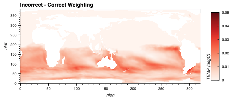
difference = yearly_average_weighted_incorrectly.TEMP - yearly_average_weighted_correctly
Since most of our values are much larger for the incorrect weigthing, we use a red colobar for that plot.
difference_plot = plot_field(difference, 'Incorrect - Correct Weighting', cmap='Reds', vmax=0.05)
We can visualize our plots stacked on top of each other, by using hv.Layout and specifying .cols(1) which will keep them in a single column.
hv.Layout([incorrect_plot, correct_plot, difference_plot]).cols(1)
Conclusion#
Time can be a tricky thing when working with Xarray - if you aren’t careful, you may be calculating your averages incorrectly!
This example covered how to efficiently calculate annual averages from monthly data, weighting by the number of days in each month.
Weighting incorrectly can cause subtle errors in your analysis, so be sure to know when to use weighted averages.