Global precipitation climatology and ITCZ migration from GPM IMERG

Run this notebook interactively on CIRRUS BinderHub.

Global precipitation climatology and the migrating tropical rain belt¶

GPM IMERG Final (monthly) is NASA’s satellite-and-gauge precipitation product. It comes from GPM, the Global Precipitation Measurement mission — an international NASA–JAXA satellite constellation that estimates rainfall worldwide — and IMERG (Integrated Multi-satellitE Retrievals for GPM), the algorithm that blends those microwave and infrared observations into a single global, 0.1° map of the monthly-mean precipitation rate. GDEX’s copy spans June 2000 – October 2025; the earliest years lean on GPM’s predecessor, TRMM (the Tropical Rainfall Measuring Mission, 1997–2015). The satellite estimates are bias-corrected against ground rain-gauge records.

In this notebook we

open the full ~25-year monthly record from GDEX,
average it in time to map the global precipitation climatology (the long-term average rainfall pattern) — revealing the Intertropical Convergence Zone (ITCZ), the band of heavy rain where the trade winds meet near the equator, along with the monsoons and the dry subtropical deserts, then
average around each latitude circle to show how that rain belt migrates north and south with the seasons.

# Imports
import os
import calendar
import numpy as np
import xarray as xr
import matplotlib.pyplot as plt
import matplotlib.animation as animation
from matplotlib.colors import BoundaryNorm
import cartopy.crs as ccrs
import cartopy.feature as cfeature

Open the dataset¶

IMERG is distributed as hundreds of monthly HDF5 granules. GDEX adds a kerchunk reference — a single JSON index recording which byte range of which granule holds each chunk — so one xr.open_dataset(..., engine="kerchunk") call presents the whole record as one virtual xarray.Dataset, and you stream only the chunks you actually use.

GDEX publishes the reference in two forms we care about:

Form	When to use it
POSIX (`/gdex/data/...`)	on a machine that mounts `/gdex/data` — NCAR HPC and CIRRUS Binder
OSDF (`...-remote-osdf.json`)	off-cluster (laptop, other hubs); chunks stream over the OSDF cache network

The cell below selects POSIX when the mount is present and falls back to OSDF, so the notebook runs unchanged in either place. The OSDF form’s chunk URLs use the osdf:// scheme, resolved by pelicanfs (installed via environment.yml; fsspec registers it automatically).

# Where to read the IMERG monthly kerchunk reference from — POSIX if the GDEX
# data mount is present, otherwise the OSDF-routed reference over the web.
posix_ref = "/gdex/data/d736000/kerchunk/GPM_3IMERGM_v07.json"
osdf_ref  = "https://data.gdex.ucar.edu/d736000/kerchunk/GPM_3IMERGM_v07-remote-osdf.json"

kerchunk_ref = posix_ref if os.path.exists(posix_ref) else osdf_ref
print(f"Access: {'POSIX mount' if kerchunk_ref == posix_ref else 'OSDF (remote)'}")
print(kerchunk_ref)

Access: POSIX mount
/gdex/data/d736000/kerchunk/GPM_3IMERGM_v07.json

Inspect the precipitation field¶

The monthly-mean rain rate lives in the precipitation variable. Two things to note before we compute:

its dimensions are ordered (time, lon, lat) — longitude before latitude — so we transpose to (lat, lon) when mapping;
its units are mm/hr; we convert to the more intuitive mm/day (× 24) for the plots.

Opening with chunks={} keeps the array lazy (Dask-backed) using the reference’s native chunking, so nothing is read until we reduce it.

ds = xr.open_dataset(kerchunk_ref, engine="kerchunk", chunks={})
precip = ds["precipitation"]        # (time, lon, lat), mm/hr
precip

Global precipitation climatology¶

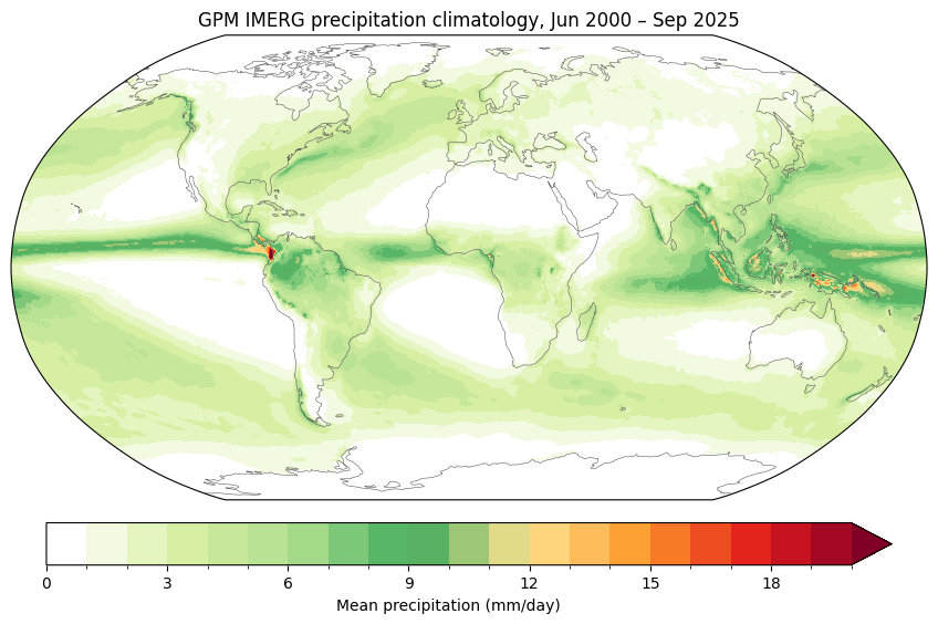
Averaging the full 304-month record gives the long-term mean rain rate at every 0.1° pixel. We convert mm/hr → mm/day for readability.

%%time
# Average over all months, then convert mm/hr -> mm/day. Result is one (lat, lon) map.
clim = precip.where(precip >= 0).mean("time")
clim = (clim * 24.0).transpose("lat", "lon")
clim.attrs["units"] = "mm/day"
clim = clim.compute()
clim

CPU times: user 1min 28s, sys: 10.5 s, total: 1min 38s
Wall time: 3min 37s

Map the climatology¶

On a global map the long-term mean highlights the ITCZ as a bright band of heavy rain near the equator, flanked by the dry subtropical deserts and ocean highs, and by the mid-latitude storm tracks.

# Shared precipitation palette: white (dry) -> greens -> warm (wet).
from matplotlib.colors import LinearSegmentedColormap

PRECIP_CMAP = LinearSegmentedColormap.from_list(
    "precip_white_warm",
    ["#ffffff", "#d9f0a3", "#addd8e", "#41ab5d",
     "#fee391", "#fe9929", "#e31a1c", "#800026"],)

print(f"range: {float(clim.min()):.2f} – {float(clim.max()):.2f} mm/day")

plot = clim.coarsen(lat=2, lon=2, boundary="trim").mean()   # 0.1° -> 0.2°, lighter figure

clim_levels = np.arange(0, 21, 1)                           # mm/day
clim_norm   = BoundaryNorm(clim_levels, PRECIP_CMAP.N, extend="max")

fig, ax = plt.subplots(figsize=(11, 5.5),
                       subplot_kw={"projection": ccrs.Robinson()},
                       constrained_layout=True)
p = ax.pcolormesh(plot["lon"], plot["lat"], plot,
                  transform=ccrs.PlateCarree(),
                  cmap=PRECIP_CMAP, norm=clim_norm,
                  shading="auto", rasterized=True)
ax.coastlines(linewidth=0.4, color="0.35")
ax.set_global()
cb = plt.colorbar(p, ax=ax, orientation="horizontal", shrink=0.7, pad=0.04, extend="max")
cb.set_label("Mean precipitation (mm/day)")
ax.set_title("GPM IMERG precipitation climatology, Jun 2000 – Sep 2025")
plt.show()

range: 0.00 – 29.05 mm/day

The seasonal cycle, animated¶

NASA’s IMERG monthly climatology shows the tropical rain belt breathing north and south across the year. We reproduce it here from the same data: twelve monthly-mean maps, played as a loop. Watch the ITCZ and the monsoons swing into the summer hemisphere each half-year.

%%time
# 12-month climatology maps (mm/day), coarsened for a light animation.
monthly = precip.where(precip >= 0).groupby("time.month").mean("time")   # (month, lon, lat)
monthly_map = (monthly * 24.0).transpose("month", "lat", "lon")
monthly_map = monthly_map.coarsen(lat=2, lon=2, boundary="trim").mean().compute()
monthly_map.attrs["units"] = "mm/day"
print("shape:", monthly_map.shape, "| max:", float(monthly_map.max()))

shape: (12, 900, 1800) | max: 45.51046371459961
CPU times: user 1min 17s, sys: 9.36 s, total: 1min 26s
Wall time: 1min 46s

anim_levels = np.arange(0, 26, 1)                           # mm/day
anim_norm   = BoundaryNorm(anim_levels, PRECIP_CMAP.N, extend="max")

lat, lon = monthly_map["lat"], monthly_map["lon"]

fig, ax = plt.subplots(figsize=(10, 5),
                       subplot_kw={"projection": ccrs.PlateCarree()},
                       constrained_layout=True)
ax.set_global()
ax.coastlines(linewidth=0.4, color="0.35")

mesh = ax.pcolormesh(lon, lat, monthly_map.isel(month=0),
                     transform=ccrs.PlateCarree(), cmap=PRECIP_CMAP, norm=anim_norm,
                     shading="auto", rasterized=True)
cb = plt.colorbar(mesh, ax=ax, orientation="horizontal", shrink=0.7, pad=0.05, extend="max")
cb.set_label("Precipitation (mm/day)")
title = ax.set_title("")

def update(m):
    mesh.set_array(monthly_map.isel(month=m).values.ravel())
    title.set_text(f"GPM IMERG climatology — {calendar.month_name[m + 1]}")
    return mesh, title

anim = animation.FuncAnimation(fig, update, frames=12, interval=700, blit=False)
plt.close(fig)

from IPython.display import HTML
HTML(anim.to_jshtml())