Trend in horizontal gradient metric

Contents

Trend in horizontal gradient metric¶

%load_ext autoreload
%autoreload 2

import numpy as np
import xarray as xr
import pandas as pd

from scipy.stats import linregress

import matplotlib.pyplot as plt

import util
import obs_surface
import figure_panels

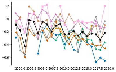
dset_djf = ds_djf.groupby('stncode').mean('record').sel(stncode=obs_surface.southern_ocean_stn_list)

fig = plt.figure()
ax = fig.add_subplot(1, 1, 1)

marker_spec = figure_panels.marker_spec_surface_stations()
x = dset_djf.time + 0.04
for i, stn_code in enumerate(dset_djf.stncode.values):

    y = dset_djf.CO2.sel(stncode=stn_code)
    ax.plot(x, y, linestyle='-', **marker_spec[stn_code])

X = DCO2y_djf.time.values
Y = DCO2y_djf.CO2.values
ax.plot(X, Y, 'ko-')

[<matplotlib.lines.Line2D at 0x2aee7027f310>]

_images/gradients-trends_7_1.png

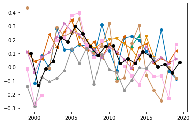
dset_jja = ds_jja.groupby('stncode').mean('record').sel(stncode=obs_surface.southern_ocean_stn_list)

fig = plt.figure()
ax = fig.add_subplot(1, 1, 1)

marker_spec = figure_panels.marker_spec_surface_stations()
x = dset_jja.time + 0.04
for i, stn_code in enumerate(dset_jja.stncode.values):

    y = dset_jja.CO2.sel(stncode=stn_code)
    ax.plot(x, y, linestyle='-', **marker_spec[stn_code])

X = DCO2y_jja.time.values
Y = DCO2y_jja.CO2.values
ax.plot(X, Y, 'ko-')

[<matplotlib.lines.Line2D at 0x2aee709b6450>]

_images/gradients-trends_8_1.png

periods = [
    (1999, 2006),
    (2005, 2020),
    (1999, 2020),    
]

lines = []
for i, period in enumerate(periods):
    dsp = DCO2y_djf.sel(time=slice(period[0], period[1]))
    d = dict(
        year_range=f"{int(dsp.time.values[0])}-{int(dsp.time.values[-1])}",
        delta=dsp.CO2.values[-1] - dsp.CO2.values[0],
    )
    d['slope'], d['intercept'], d['r_value'], d['p_value'], d['stderr'] = linregress(dsp.time,  dsp.CO2)
    lines.append(d)
df_fit_djf = pd.DataFrame(lines).set_index("year_range")
df_fit_djf

	delta	slope	intercept	r_value	p_value	stderr
year_range
1999-2005	0.052332	0.015879	-31.939016	0.235028	0.611932	0.029369
2005-2019	-0.179887	-0.014225	28.425354	-0.780448	0.000597	0.003161
1999-2019	-0.127555	-0.006835	13.545181	-0.412210	0.063331	0.003466

lines = []
for i, period in enumerate(periods):
    dsp = DCO2y_jja.sel(time=slice(period[0], period[1]))
    d = dict(
        year_range=f"{int(dsp.time.values[0])}-{int(dsp.time.values[-1])}",
        delta=dsp.CO2.values[-1] - dsp.CO2.values[0],
    )
    d['slope'], d['intercept'], d['r_value'], d['p_value'], d['stderr'] = (
        linregress(dsp.time,  dsp.CO2)
    )
    lines.append(d)
df_fit_jja = pd.DataFrame(lines).set_index("year_range")
df_fit_jja

	delta	slope	intercept	r_value	p_value	stderr
year_range
1999-2005	0.198383	0.052205	-104.442431	0.764587	0.045284	0.019680
2005-2019	-0.262310	-0.017257	34.823807	-0.831013	0.000124	0.003204
1999-2019	-0.063927	-0.003656	7.432276	-0.222359	0.332654	0.003677

Mean changes over 2005-2019¶

(df_fit_djf[["delta", "slope", "stderr"]].loc["2005-2019"] + df_fit_jja[["delta", "slope", "stderr"]].loc["2005-2019"])/2

delta    -0.221098
slope    -0.015741
stderr    0.003182
Name: 2005-2019, dtype: float64

previous

Seasonal amplitude of vertical gradient

next

Aircraft atmospheric CO₂ profiles