Observed patterns in atmospheric CO₂¶

We use observations from nine deployments of three recent aircraft projects: the HIAPER Pole-to-Pole Observations (HIPPO) project [Wofsy and HIPPO Science Team and Cooperating Modellers and Satellite Teams, 2011]; the O₂/N₂ Ratio and CO₂ Airborne Southern Ocean (ORCAS) study [Stephens et al., 2018]; and the Atmospheric Tomography (ATom) mission [Wofsy et al., 2018].

We also examined 44 atmospheric CO₂ records from surface monitoring stations in the high-latitude Southern Hemisphere, selecting and filtering the highest quality data.

This notebook creates a figure summarizing these data. Additional details are provided in other notebooks:

%load_ext autoreload
%autoreload 2

import numpy as np

import matplotlib.pyplot as plt
import matplotlib.gridspec as gridspec
from matplotlib.lines import Line2D

import util
import figure_panels
import datasets

config warning: cannot mkdir /glade/work/mclong/so-co2-airborne-obs
setting project_tmpdir to /Users/mclong/scratch/tmp/so-co2-airborne-obs/project_tmpdir
config warning: cannot mkdir /glade/work/mclong/so-co2-airborne-obs
setting project_tmpdir to /Users/mclong/scratch/tmp/so-co2-airborne-obs/project_tmpdir
config warning: cannot mkdir /glade/work/mclong/so-co2-airborne-obs
setting project_tmpdir to /Users/mclong/scratch/tmp/so-co2-airborne-obs/project_tmpdir

Load obervational datasets¶

Here we make use of functions provided by the datasets module; see API documentation for additional details.

%%time
dsets = dict(
    ds_obs_aircraft=datasets.aircraft_sections(),
    ds_obs_srf_djf=datasets.obs_surface_stn_v_lat('djf'),
    ds_obs_srf_jja=datasets.obs_surface_stn_v_lat('jja'),
)
dsets

CPU times: user 348 ms, sys: 14.9 ms, total: 363 ms
Wall time: 363 ms

{'ds_obs_aircraft': <xarray.Dataset>
 Dimensions:       (z: 22, y: 20, time: 9, ye: 20, ze: 23)
 Coordinates:
     ALT           (z, y) float64 0.25 0.25 0.25 0.25 ... 10.75 10.75 10.75 10.75
     LAT           (z, y) float64 -78.75 -76.25 -73.75 ... -36.25 -33.75 -31.25
     campaigns     (time) <U7 'HIPPO-1' 'HIPPO-2' 'HIPPO-3' ... 'ATom-3' 'ATom-4'
     month         (time) int64 1 11 4 8 2 8 2 10 5
   * time          (time) datetime64[ns] 2009-01-20 2009-11-11 ... 2018-05-07
   * y             (y) float64 -78.75 -76.25 -73.75 ... -36.25 -33.75 -31.25
   * ye            (ye) float64 -80.0 -77.5 -75.0 -72.5 ... -37.5 -35.0 -32.5
     year          (time) int64 2009 2009 2010 2011 2016 2016 2017 2017 2018
   * z             (z) float64 0.25 0.75 1.25 1.75 2.25 ... 9.25 9.75 10.25 10.75
   * ze            (ze) float64 0.0 0.5 1.0 1.5 2.0 ... 9.0 9.5 10.0 10.5 11.0
 Data variables:
     CO2_binned    (time, z, y) float64 nan nan nan nan ... 406.0 405.9 405.6
     DCO2_binned   (time, z, y) float64 nan nan nan nan ... 1.148 1.03 0.7236
     N_CO2         (time, z, y) float64 nan nan nan nan ... 56.0 209.0 252.0 66.0
     N_DCO2        (time, z, y) float64 nan nan nan nan ... 56.0 209.0 252.0 66.0
     THETA         (time, z, y) float64 nan nan nan nan ... 327.8 336.2 336.9
     THETA_binned  (time, z, y) float64 nan nan nan nan ... 327.3 336.5 337.4,
 'ds_obs_srf_djf': <xarray.Dataset>
 Dimensions:      (record: 32, time: 22)
 Coordinates:
   * record       (record) object 'SPO_NOAA_insitu_CO2' ... 'CPT_SAWS_insitu_CO2'
     institution  (record) object 'NOAA' 'NOAA' 'SIO_O2' ... 'NOAA' 'LSCE' 'SAWS'
     lat          (record) float64 -89.98 -89.98 -89.98 ... -40.68 -37.8 -34.35
     lon          (record) float64 -24.8 -24.8 -24.8 -24.8 ... 144.7 77.54 18.49
     stncode      (record) object 'SPO' 'SPO' 'SPO' 'SPO' ... 'CGO' 'AMS' 'CPT'
   * time         (time) int64 1999 2000 2001 2002 2003 ... 2017 2018 2019 2020
 Data variables:
     CO2          (time, record) float64 0.0 0.1004 0.02747 ... nan nan nan,
 'ds_obs_srf_jja': <xarray.Dataset>
 Dimensions:      (record: 32, time: 21)
 Coordinates:
   * record       (record) object 'SPO_NOAA_insitu_CO2' ... 'CPT_SAWS_insitu_CO2'
     institution  (record) object 'NOAA' 'NOAA' 'SIO_O2' ... 'NOAA' 'LSCE' 'SAWS'
     lat          (record) float64 -89.98 -89.98 -89.98 ... -40.68 -37.8 -34.35
     lon          (record) float64 -24.8 -24.8 -24.8 -24.8 ... 144.7 77.54 18.49
     stncode      (record) object 'SPO' 'SPO' 'SPO' 'SPO' ... 'CGO' 'AMS' 'CPT'
   * time         (time) int64 1999 2000 2001 2002 2003 ... 2016 2017 2018 2019
 Data variables:
     CO2          (time, record) float64 0.0 -0.07697 -0.0542 ... 0.03813 nan}

# set up canvas
fig = plt.figure() #figsize=(10, 6)) #dpi=300)

#------------------------------------
#--- ORCAS Section
#------------------------------------

ds = dsets['ds_obs_aircraft']
ax = fig.add_subplot(1, 1, 1) #axs['section_DJF']

ndx = np.where(ds.campaigns == 'ORCAS')[0][0]
cf = ax.pcolormesh(
        ds.y, ds.z, ds.DCO2_binned.isel(time=ndx).squeeze(),
        norm=figure_panels.divnorm,
        cmap=figure_panels.cmap,
        shading='nearest',    
    )
cs = ax.contour(
    ds.LAT, ds.ALT, ds.THETA.isel(time=ndx).squeeze(),
    levels=np.arange(255., 350., 5.),
    linewidths=1,
    colors='gray')    
lb = plt.clabel(cs, fontsize=8, inline=True, fmt='%d')  

ax.set_title('Aircraft obs: CO$_2$ minus 295–305K mean (Jan-Feb 2016)')
ax.set_ylim((0, 10.5))
ax.set_xlim(-91.25, -28.75)
ax.set_ylabel('Altitude [km]');   
ax.set_xlabel('Latitude [°N]')


cb = plt.colorbar(cf)
cb.set_label('$\Delta$CO$_2$ [ppm]')

util.savefig('co2-orcas-cross-section')

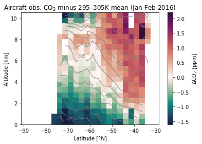
Fig. 1: Observed CO₂ distributions over the Southern Ocean¶

%%time
# set up canvas
fig = plt.figure(figsize=(10, 6)) #dpi=300)

# set up plot grid
gs_top = gridspec.GridSpec(nrows=1, ncols=3, 
                        width_ratios=(1, 1, 0.02), 
                        left=0, right=1, bottom=0.52, top=1.,
                        hspace=0.2, wspace=0.1,
                       )

gs_bot = gridspec.GridSpec(nrows=1, ncols=3, 
                        width_ratios=(1, 1, 0.02), 
                        left=0, right=1, bottom=0, top=0.4,
                        hspace=0.2, wspace=0.1,
                       )

axs = dict(
    section_DJF=plt.subplot(gs_top[0, 0]),
    section_JJA=plt.subplot(gs_top[0, 1]),
    surface_DJF=plt.subplot(gs_bot[0, 0]),
    surface_JJA=plt.subplot(gs_bot[0, 1]),        
)
caxs = dict(
    section=plt.subplot(gs_top[:, -1]),
)

#------------------------------------
#--- ORCAS Section
#------------------------------------

ds = dsets['ds_obs_aircraft']
ax = axs['section_DJF']

ndx = np.where(ds.campaigns == 'ORCAS')[0][0]
cf = ax.pcolormesh(
        ds.y, ds.z, ds.DCO2_binned.isel(time=ndx).squeeze(),
        norm=figure_panels.divnorm,
        cmap=figure_panels.cmap,
        shading='nearest',    
    )
cs = ax.contour(
    ds.LAT, ds.ALT, ds.THETA.isel(time=ndx).squeeze(),
    levels=np.arange(255., 350., 5.),
    linewidths=1,
    colors='gray')    
lb = plt.clabel(cs, fontsize=8, inline=True, fmt='%d')  

ax.set_title('Aircraft obs: CO$_2$ minus 295–305K mean (Jan-Feb 2016)')
ax.set_ylim((0, 10.5))
ax.set_xlim(-91.25, -28.75)
ax.set_ylabel('Altitude [km]')        


#------------------------------------
#--- ATom Section
#------------------------------------

ds = dsets['ds_obs_aircraft']
ax = axs['section_JJA']

ndx = np.where(ds.campaigns == 'ATom-1')[0][0]
cf = ax.pcolormesh(
        ds.y, ds.z, ds.DCO2_binned.isel(time=ndx).squeeze(),
        norm=figure_panels.divnorm,
        cmap=figure_panels.cmap,
        shading='nearest',
    )
cs = ax.contour(
    ds.LAT, ds.ALT, ds.THETA.isel(time=ndx).squeeze(),
    levels=np.arange(255., 350., 5.),
    linewidths=1,
    colors='gray')    
lb = plt.clabel(cs, fontsize=8, inline=True, fmt='%d') 

ax.set_title('Aircraft obs: CO$_2$ minus 295–305K mean (Aug 2016)')
ax.set_ylim((0, 10.5))
ax.set_xlim(-91.25, -28.75)
ax.set_yticklabels([])

cax = caxs['section']
plt.colorbar(cf, cax=cax)
cax.set_title('$\Delta$CO$_2$ [ppm]', loc='left')

#------------------------------------
#--- DJF Surface
#------------------------------------

ds = dsets['ds_obs_srf_djf']
ax = axs[f'surface_DJF']
figure_panels.stn_v_lat(ds.CO2, ax)   
ax.set_ylabel('')
ax.set_title(f'Surface obs: DJF CO$_2$ minus SPO (1999-2019)')
ax.set_xlim(-91.25, -28.75)
ax.set_ylabel('$\Delta_{ y}$CO$_2$ [ppm]')

#------------------------------------
#--- JJA Surface
#------------------------------------

ds = dsets['ds_obs_srf_jja']
ax = axs[f'surface_JJA']
figure_panels.stn_v_lat(ds.CO2, ax)   
ax.set_ylabel('')
ax.set_title(f'Surface obs: JJA CO$_2$ minus SPO (1999-2019)')
ax.set_xlim(-91.25, -28.75)
ax.set_yticklabels([])


marker_spec = figure_panels.marker_spec_co2_inst()
legend_elements = [Line2D([0], [0], label=inst, linestyle=None, **spec) 
                   for inst, spec in marker_spec.items() if inst != 'Multiple']
ax.legend(handles=legend_elements, ncol=1, 
          fontsize=8, loc=(1.02, 0), frameon=False);

plot_keys = [
    'section_DJF', 'section_JJA', 
    'surface_DJF', 'surface_JJA', 
]   
util.label_plots(fig, [axs[k] for k in plot_keys], xoff=-0.02, yoff=0.02)

util.savefig(f'co2-aircraft-surface-obs')

CPU times: user 4.48 s, sys: 101 ms, total: 4.58 s
Wall time: 2.14 s

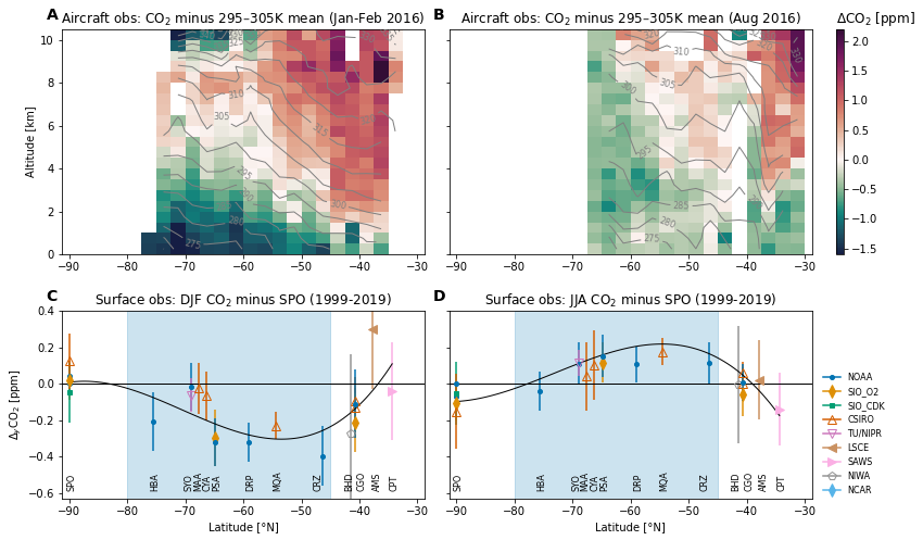
Observed patterns in atmospheric CO₂ over the Southern Ocean. Observed patterns in atmospheric CO₂ over the Southern Ocean. Upper panels: Cross-sections observed by aircraft during (A) ORCAS, Jan–Feb 2016 and (B) ATom-1, Aug 2016. Colors show the observed CO₂ dry air mole fraction relative to the average observed within the 295–305 K potential temperature range south of 45°S on each campaign; contour lines show the observed potential temperature. Fight-tracks and cross-section plots for all campaigns are shown here and this notebook illustrates the distributions of CO₂ simulated by a 3-D transport model. Lower panels: Compilation of mean CO₂ observed at surface monitoring stations minus the NOAA in situ record at the South Pole Observatory (SPO) over 1999–2019 for (C) summer (DJF) and (D) winter (JJA). The black line is a spline fit provided simply as a visual guide. Blue shading denotes the latitude band in which we designate “Southern Ocean stations.” Station locations and temporal coverage are shown here.

Strong Southern Ocean Carbon Uptake Evident in Airborne Observations

Observed patterns in atmospheric CO₂

Contents

Observed patterns in atmospheric CO₂¶

Load obervational datasets¶

Fig. 1: Observed CO₂ distributions over the Southern Ocean¶

Strong Southern Ocean Carbon Uptake Evident in Airborne Observations

Observed patterns in atmospheric CO2

Contents

Observed patterns in atmospheric CO2¶

Load obervational datasets¶

Fig. 1: Observed CO2 distributions over the Southern Ocean¶

Observed patterns in atmospheric CO₂

Observed patterns in atmospheric CO₂¶

Fig. 1: Observed CO₂ distributions over the Southern Ocean¶