The spell mini-language

A “spell” compresses a whole processing chain into one string, so a diagnostic can live in a config file or a plot title.

[alias ~] variable[.isel(...)][|modifiers] : temporal : spatial

import os
import numpy as np
import xarray as xr
import matplotlib.pyplot as plt
import nc_time_axis  # registers the cftime axis converter for matplotlib
import x4c

x4c.set_style('journal')

# after set_style: it resets rcParams from matplotlibrc defaults, which includes the
# backend, so assert the inline backend last or figures are never captured
%matplotlib inline

# The tutorial runs against a reduced copy of a real CESM case. It is published as a
# GitHub Release asset rather than committed, so the first call downloads it into
# ~/.cache/x4c (override with $X4C_CACHE_DIR) and later calls reuse it. Set
# $X4C_SAMPLE_DIR to point at a copy you already have.
case_dir = x4c.fetch_sample_data(case='cesm1', verbose=False)
casename = os.path.basename(case_dir)
print('x4c', x4c.__version__)

x4c 2026.6.11

from x4c import Spell

case = x4c.Timeseries(case_dir, grid_dict={'atm': 'ne16np4', 'ocn': 'g16'}, cesm_ver=1)

>>> case.root_dir: /glade/u/home/fengzhu/.cache/x4c/sample_data/cesm1_sample_data/b.e13.B1850C5.ne16_g16.icesm131_d18O_fixer.Miocene.3xCO2.005
>>> case.path_pattern: comp/proc/tseries/*/casename.hstr.vn.timespan.nc
>>> case.grid_dict: {'atm': 'ne16np4', 'ocn': 'g16', 'lnd': 'ne16np4', 'rof': 'ne16np4', 'ice': 'g16'}
>>> case.casename: b.e13.B1850C5.ne16_g16.icesm131_d18O_fixer.Miocene.3xCO2.005
>>> case.paths["atm"]["cam.h0"] created
>>> case.paths["ocn"]["pop.h"] created
>>> case.paths["lnd"]["clm2.h0"] created
>>> case.paths["ice"]["cice.h"] created
>>> case.vns["atm"]["cam.h0"] created
>>> case.vns["ocn"]["pop.h"] created
>>> case.vns["lnd"]["clm2.h0"] created
>>> case.vns["ice"]["cice.h"] created

Parsing¶

A Spell is parsed, not evaluated. Arguments are read with a restricted parser that accepts numbers, strings, containers and slice(...) — and nothing else — so a spell from an untrusted config cannot execute code.

S = Spell('GMST ~ TS:ann:gm')
print(S)
print()
print('alias      :', S.alias)
print('variable   :', S.vn)
print('temporal   :', S.ann_method)
print('spatial    :', S.sa_method)

Spell(vn='TS', alias='GMST', ann_method='ann', sa_method='gm')

alias      : GMST
variable   : TS
temporal   : ann
spatial    : gm

S = Spell('T.isel(lev=-1)|regrid(2,2)|plev(500,850):climo:zm')
for f in ['vn', 'slicing_method', 'slicing_kwargs', 'regrid_args',
          'plev_levels', 'ann_method', 'sa_method']:
    print(f'{f:16s} {getattr(S, f)!r}')

vn               'T'
slicing_method   'isel'
slicing_kwargs   {'lev': -1}
regrid_args      (2, 2)
plev_levels      [500, 850]
ann_method       'climo'
sa_method        'zm'

Malformed spells fail at parse time, naming the spell, rather than part-way through a long computation.

for bad in ['TS:ann:gm:extra', 'TS:ann:not_a_method', 'TS|regrid(open("x")):ann']:
    try:
        Spell(bad)
    except ValueError as e:
        print(f'{bad:38s} -> {str(e)[:80]}')

TS:ann:gm:extra                        -> Cannot parse spell `TS:ann:gm:extra`: expected at most 3 colon-separated fields 
TS:ann:not_a_method                    -> Unknown spatial average method `not_a_method` in spell `TS:ann:not_a_method`. Op
TS|regrid(open("x")):ann               -> Cannot call `open` in `regrid(open("x"))`: the only callable allowed in a spell

Computing a spell¶

case.calc(spell) runs the chain and caches the result under case.diags[spell].

gmst = case.calc('GMST ~ TS:ann:gm', timespan=(1, 10))
print(dict(gmst.sizes))
print(np.round(gmst.values, 3))

>>> case.ds["TS"] created
>>> Timespan: [0001-01-01 00:00:00, 0010-12-01 00:00:00]

>>> case.diags["GMST"] created
{'time': 10}
[23.245 23.204 23.358 23.354 23.065 23.123 23.237 23.367 23.025 22.849]

Note the units: calc converts a field tagged K to degrees Celsius.

print('name :', gmst.name)
print('units:', gmst.attrs.get('units'))
print('cached under:', [k for k in case.diags])

name : GMST
units: °C
cached under: ['GMST']

A few spells at once¶

This is where the notation pays off — a diagnostics suite becomes a dictionary.

spells = {
    'GMST': 'TS:ann:gm',
    'GMPRECT': 'PRECT:ann:gm',
    'RESTOM': 'RESTOM:ann:gm',
    'NHICE': 'ICEFRAC:ann:nhm',
}
for key, spell in spells.items():
    case.calc(spell, timespan=(1, 10), verbose=False)
    print(f'{key:8s} {spell:22s} -> {np.round(case.diags[spell].values, 3)}')

>>> Timespan: [0001-01-01 00:00:00, 0010-12-01 00:00:00]

GMST     TS:ann:gm              -> [23.245 23.204 23.358 23.354 23.065 23.123 23.237 23.367 23.025 22.849]
>>> Timespan: [0001-01-01 00:00:00, 0010-12-01 00:00:00]

GMPRECT  PRECT:ann:gm           -> [0. 0. 0. 0. 0. 0. 0. 0. 0. 0.]
>>> Timespan: [0001-01-01 00:00:00, 0010-12-01 00:00:00]

RESTOM   RESTOM:ann:gm          -> [ 0.146 -0.118  0.254  0.269  0.863  1.29   0.425  0.753  0.097  1.095]
>>> Timespan: [0001-01-01 00:00:00, 0010-12-01 00:00:00]

NHICE    ICEFRAC:ann:nhm        -> [0. 0. 0. 0. 0. 0. 0. 0. 0. 0.]

fig, axes = plt.subplots(2, 2, figsize=(11, 5.5))
for axi, (key, spell) in zip(axes.ravel(), spells.items()):
    d = case.diags[spell]
    axi.plot(d.time, d.values, marker='o', ms=3)
    axi.set(title=key, ylabel=d.attrs.get('units', ''))
fig.tight_layout()
x4c.showfig(fig)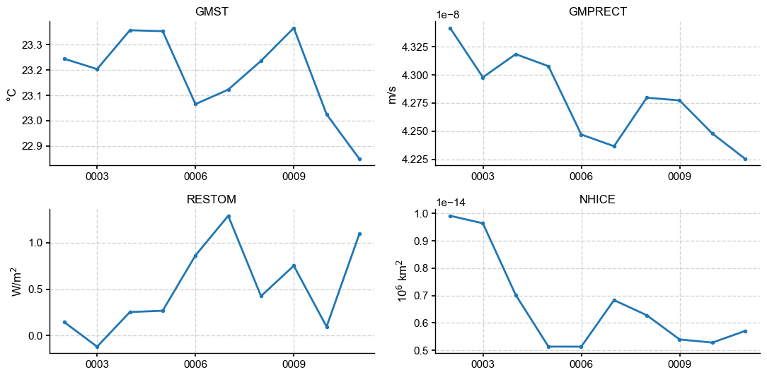

Spells with modifiers¶

|regrid puts the field on a regular grid before the spatial step; .isel(...) slices the variable first. The ocean 3-D fields in the sample cover year 1 only.

sst = case.calc('SST ~ TEMP.isel(z_t=0)|regrid(2,2):climo', timespan=(1, 1))
print(dict(sst.sizes))

>>> case.ds["TEMP"] created
>>> Timespan: [0001-01-01 00:00:00, 0001-12-01 00:00:00]

>>> case.diags["SST"] created
{'time': 12, 'lat': 90, 'lon': 180}

ssh_path = os.path.join(case_dir, 'ocn', 'proc', 'tseries', 'month_1',
                        f'{casename}.pop.h.SSH.000101-000512.nc')
ssv = x4c.open_dataset(ssh_path, comp='ocn', grid='g16', vn='SSH',
                       shift_time=True).x.regrid().x.da.mean('time')

fig, ax = sst.mean('time').x.plot(ssv=ssv, title='Sea-surface temperature (year 1)')
x4c.showfig(fig)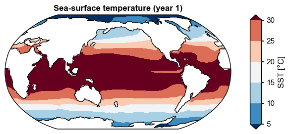

`zavg`: a depth-weighted average¶

|zavg(top, bottom) averages over a depth range in the units of z_t (centimetres for POP). It folds the layer thicknesses into the area weight, so a following gm gives a true volume-weighted mean rather than a depth-mean of area-means.

The sample keeps only the upper ocean levels, so use a shallow range.

upper = case.calc('T100 ~ TEMP|zavg(0,10000):ann:gm', timespan=(1, 1))
print('volume-mean temperature, top 100 m:', np.round(upper.values, 3),
      upper.attrs.get('units'))

>>> case.ds["TEMP"] already loaded; to reload, run case.load("TEMP", ..., reload=True).
>>> Timespan: [0001-01-01 00:00:00, 0001-12-01 00:00:00]

>>> case.diags["T100"] created
volume-mean temperature, top 100 m: 23.808 °C

Derived variables¶

A spell doesn’t have to name a variable that exists on disk. case.calc first checks whether the name is a registered derived diagnostic (see x4c.diags.Registry) and, if so, loads whatever raw variables it needs and combines them — LST (land-only surface temperature) masks TS with LANDFRAC; d18Op combines the eight isotopic precipitation fluxes into a single per-mil ratio.

lst = case.calc('LST:ann:gm', timespan=(1, 10))
d18o = case.calc('d18Op:ann:gm', timespan=(1, 10))
print('LST  :', np.round(lst.values, 3), lst.attrs.get('units'))
print('d18Op:', np.round(d18o.values, 3), d18o.attrs.get('units'))

>>> LST is a supported derived variable.
>>> case.ds["TS"] already loaded; to reload, run case.load("TS", ..., reload=True).
>>> case.ds["LANDFRAC"] created
>>> case.ds["LST"] created
>>> Timespan: [0001-01-01 00:00:00, 0010-12-01 00:00:00]

>>> case.diags["LST:ann:gm"] created
>>> d18Op is a supported derived variable.
>>> case.ds["PRECRC_H216Or"] created
>>> case.ds["PRECSC_H216Os"] created
>>> case.ds["PRECRL_H216OR"] created

>>> case.ds["PRECSL_H216OS"] created
>>> case.ds["PRECRC_H218Or"] created
>>> case.ds["PRECSC_H218Os"] created

>>> case.ds["PRECRL_H218OR"] created
>>> case.ds["PRECSL_H218OS"] created
>>> case.ds["d18Op"] created
>>> Timespan: [0001-01-01 00:00:00, 0010-12-01 00:00:00]

>>> case.diags["d18Op:ann:gm"] created
LST  : [17.063 17.715 17.962 17.989 17.59  17.753 18.051 18.106 17.658 17.457] °C
d18Op: [-5.4   -5.648 -5.642 -5.65  -5.718 -5.635 -5.623 -5.667 -5.726 -5.738] permil

A horizontal map¶

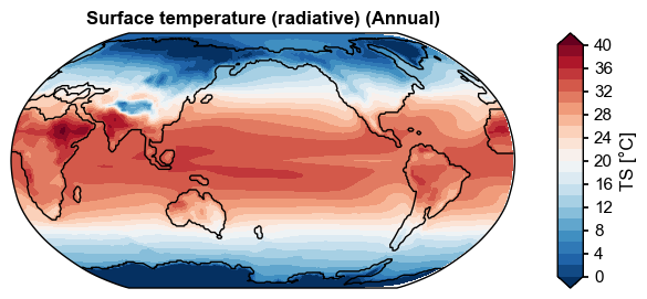
Skip the spatial-average field and case.plot renders a map for the last timestep instead — TS:ann keeps the ncol dimension around.

spell = 'TS:ann'
case.calc(spell, timespan=(1, 10))
fig, ax = case.plot(spell)
x4c.showfig(fig)

>>> case.ds["TS"] already loaded; to reload, run case.load("TS", ..., reload=True).
>>> Timespan: [0001-01-01 00:00:00, 0010-12-01 00:00:00]

>>> case.diags["TS:ann"] created

>>> case.ds["SSH"] created

A zonal mean¶

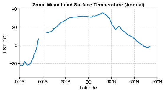
:zm collapses longitude (or ncol), leaving (time, lat).

spell = 'LST:ann:zm'
case.calc(spell, timespan=(1, 10))
fig, ax = case.plot(spell)
x4c.showfig(fig)

>>> LST is a supported derived variable.
>>> case.ds["TS"] already loaded; to reload, run case.load("TS", ..., reload=True).
>>> case.ds["LANDFRAC"] already loaded; to reload, run case.load("LANDFRAC", ..., reload=True).
>>> case.ds["LST"] created
>>> Timespan: [0001-01-01 00:00:00, 0010-12-01 00:00:00]

>>> case.diags["LST:ann:zm"] created

A vertical section¶

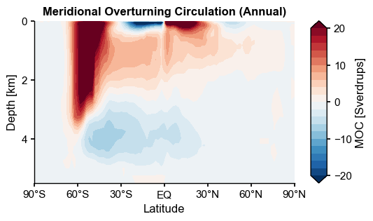
:yz keeps a (lat, z_t) cross-section — MOC is a good example, since it is naturally defined on that plane.

spell = 'MOC:ann:yz'
case.calc(spell, timespan=(1, 10))
fig, ax = case.plot(spell)
x4c.showfig(fig)

>>> MOC is a supported derived variable.
>>> case.ds["MOC"] created
>>> Timespan: [0001-01-01 00:00:00, 0010-12-01 00:00:00]

>>> case.diags["MOC:ann:yz"] created

Combining two spells¶

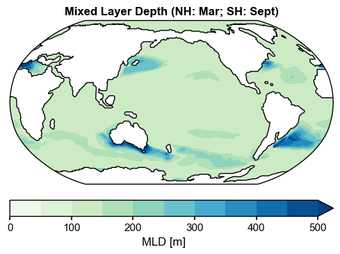
A spell result is just an xr.DataArray, so nothing stops combining several of them with plain xarray — here .where() stitches a hemisphere-appropriate mixed-layer depth from the March and September climatologies (MLD:3, MLD:9) and stores the result back into case.diags under a new key so it plots like any other spell.

case.calc('MLD:3', timespan=(1, 10))
case.calc('MLD:9', timespan=(1, 10))

mask = case.diags['MLD:3'].lat > 0
case.diags['MLD:mix'] = case.diags['MLD:3'].mean('time').where(
    mask, other=case.diags['MLD:9'].mean('time'))

fig, ax = case.plot(
    'MLD:mix',
    figsize=(6, 6),
    cbar_kwargs={'orientation': 'horizontal', 'aspect': 20, 'pad': 0.05},
)
ax.set_title('Mixed Layer Depth (NH: Mar; SH: Sept)', weight='bold')
x4c.showfig(fig)

>>> MLD is a supported derived variable.

>>> case.ds["XMXL"] created
>>> case.ds["MLD"] created
>>> Timespan: [0001-01-01 00:00:00, 0010-12-01 00:00:00]
>>> case.diags["MLD:3"] created
>>> MLD is a supported derived variable.
>>> case.ds["XMXL"] already loaded; to reload, run case.load("XMXL", ..., reload=True).
>>> case.ds["MLD"] created
>>> Timespan: [0001-01-01 00:00:00, 0010-12-01 00:00:00]

>>> case.diags["MLD:9"] created