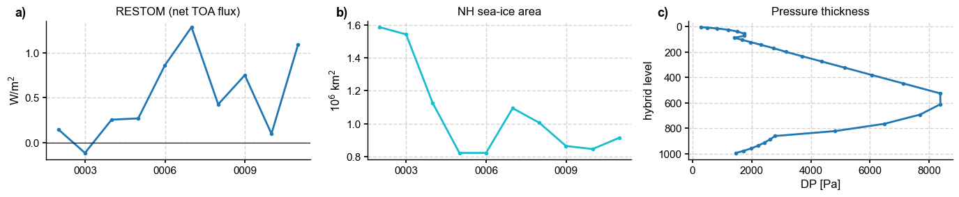
Radiation, sea ice, and climate indices

RESTOM is the net top-of-atmosphere flux (FSNT - FLNT) and is the standard equilibrium check. ICEFRAC converts sea-ice fraction into an area. DP is the pressure thickness of each hybrid layer, built from the hybrid coefficients. NINO3.4 is registered under a dotted name, which is why the decorator takes an explicit name=. It resolves like any other variable.

import os
import numpy as np
import xarray as xr
import matplotlib.pyplot as plt
import nc_time_axis  # registers the cftime axis converter for matplotlib
import x4c

x4c.set_style('journal')

# after set_style: it resets rcParams from matplotlibrc defaults, which includes the
# backend, so assert the inline backend last or figures are never captured
%matplotlib inline

# The tutorial runs against a reduced copy of a real CESM case. It is published as a
# GitHub Release asset rather than committed, so the first call downloads it into
# ~/.cache/x4c (override with $X4C_CACHE_DIR) and later calls reuse it. Set
# $X4C_SAMPLE_DIR to point at a copy you already have.
case_dir = x4c.fetch_sample_data(case='cesm1', verbose=False)
casename = os.path.basename(case_dir)
print('x4c', x4c.__version__)

x4c 2026.6.11

from x4c import diags

case = x4c.Timeseries(case_dir, grid_dict={'atm': 'ne16np4', 'ocn': 'g16'},
                      cesm_ver=1)

>>> case.root_dir: /glade/u/home/fengzhu/.cache/x4c/sample_data/cesm1_sample_data/b.e13.B1850C5.ne16_g16.icesm131_d18O_fixer.Miocene.3xCO2.005
>>> case.path_pattern: comp/proc/tseries/*/casename.hstr.vn.timespan.nc
>>> case.grid_dict: {'atm': 'ne16np4', 'ocn': 'g16', 'lnd': 'ne16np4', 'rof': 'ne16np4', 'ice': 'g16'}
>>> case.casename: b.e13.B1850C5.ne16_g16.icesm131_d18O_fixer.Miocene.3xCO2.005
>>> case.paths["atm"]["cam.h0"] created
>>> case.paths["ocn"]["pop.h"] created
>>> case.paths["lnd"]["clm2.h0"] created
>>> case.paths["ice"]["cice.h"] created
>>> case.vns["atm"]["cam.h0"] created
>>> case.vns["ocn"]["pop.h"] created
>>> case.vns["lnd"]["clm2.h0"] created
>>> case.vns["ice"]["cice.h"] created

for vn, span in [('RESTOM', (1, 10)), ('ICEFRAC', (1, 10)), ('DP', (1, 10))]:
    case.load(vn, timespan=span, verbose=False)
    da = case.ds[vn]
    print(f'  {vn:8s} {str(dict(da.sizes)):48s} {da.attrs.get("units")}')

  RESTOM   {'time': 120, 'ncol': 13826}                     W/m$^2$
  ICEFRAC  {'time': 120, 'nj': 384, 'ni': 320}              10$^6$ km$^2$
  DP       {'lev': 30, 'time': 120, 'ncol': 13826}          Pa

fig, axes = plt.subplots(1, 3, figsize=(14, 3))

restom = case.calc('RESTOM:ann:gm', timespan=(1, 10), verbose=False)
axes[0].plot(restom.time, restom, marker='o', ms=3)
axes[0].axhline(0, color='k', lw=0.8)
axes[0].set(title='RESTOM (net TOA flux)', ylabel=restom.attrs.get('units'))

ice = case.calc('ICEFRAC:ann:nhs', timespan=(1, 10), verbose=False)
axes[1].plot(ice.time, ice, marker='o', ms=3, color='tab:cyan')
axes[1].set(title='NH sea-ice area', ylabel=ice.attrs.get('units'))

dp = case.ds['DP'].x.da.isel(time=0).x.gm if 'gw' in case.ds['DP'].x.da.attrs \
    else case.ds['DP'].x.da.isel(time=0).mean('ncol')
axes[2].plot(dp.values, dp['lev'].values, marker='.')
axes[2].invert_yaxis()
axes[2].set(title='Pressure thickness', xlabel='DP [Pa]', ylabel='hybrid level')

x4c.add_annotation(list(axes), style=')', loc_x=-0.12, fs=13)
fig.tight_layout()
x4c.showfig(fig)

>>> Timespan: [0001-01-01 00:00:00, 0010-12-01 00:00:00]

>>> Timespan: [0001-01-01 00:00:00, 0010-12-01 00:00:00]

Climate indices¶

case.load('NINO3.4', timespan=(1, 1), verbose=False)
nino = case.ds['NINO3.4']
print('NINO3.4:', dict(nino.sizes), '|', nino.attrs.get('units'))
print(np.round(nino.values, 3))

NINO3.4: {'time': 12} | °C

[34.712 34.133 33.067 32.375 32.397 32.087 31.654 30.519 29.928 30.413
 30.818 31.103]

Note the units are °C, not K. That matters: Timeseries.calc subtracts 273.15 from anything labelled K, which would silently offset an index by that amount. When you add your own diagnostic, label differences, anomalies and indices with their real units — see Adding a derived variable.